Download
1 / 6
60 likes | 262 Views
Example of Newton’s Interpolating Polynomials Dr. Ferri. Try to interpolate the value of cos(0.3) using computed data points. i. x i. f[x i ]. f[x i ,x i+1 ]. f[x i ,x i+1 ,x i+2 ]. f[x i ,…x i+3 ]. f[x 0 ,…x 4 ]. 1.0000e+000 -9.9667e-002 -4.8840e-001 4.9008e-002 3.8122e-002

E N D
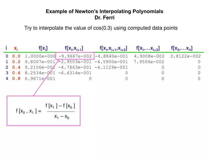
Example of Newton’s Interpolating Polynomials Dr. Ferri Try to interpolate the value of cos(0.3) using computed data points i xi f[xi] f[xi,xi+1] f[xi,xi+1,xi+2] f[xi,…xi+3] f[x0,…x4] 1.0000e+000 -9.9667e-002 -4.8840e-001 4.9008e-002 3.8122e-002 9.8007e-001 -2.9503e-001 -4.5900e-001 7.9506e-002 0 9.2106e-001 -4.7863e-001 -4.1129e-001 0 0 8.2534e-001 -6.4314e-001 0 0 0 6.9671e-001 0 0 0 0 0 1 2 3 4 0.0 0.2 0.4 0.6 0.8 f [x1 ] – f [x0 ] f [x0 , x1 ] = x1 – x0
Example of Newton’s Interpolating Polynomials Try to interpolate the value of cos(0.3) using computed data points i xi f[xi] f[xi,xi+1] f[xi,xi+1,xi+2] f[xi,…xi+3] f[x0,…x4] 1.0000e+000 -9.9667e-002 -4.8840e-001 4.9008e-002 3.8122e-002 9.8007e-001 -2.9503e-001 -4.5900e-001 7.9506e-002 0 9.2106e-001 -4.7863e-001 -4.1129e-001 0 0 8.2534e-001 -6.4314e-001 0 0 0 6.9671e-001 0 0 0 0 0 1 2 3 4 0.0 0.2 0.4 0.6 0.8 f [x1, x2 ] – f [x0, x1 ] f [x0 , x1 , x2] = x2 – x0
Example of Newton’s Interpolating Polynomials Try to interpolate the value of cos(0.3) using computed data points i xi f[xi] f[xi,xi+1] f[xi,xi+1,xi+2] f[xi,…xi+3] f[x0,…x4] 1.0000e+000 -9.9667e-002 -4.8840e-001 4.9008e-002 3.8122e-002 9.8007e-001 -2.9503e-001 -4.5900e-001 7.9506e-002 0 9.2106e-001 -4.7863e-001 -4.1129e-001 0 0 8.2534e-001 -6.4314e-001 0 0 0 6.9671e-001 0 0 0 0 0 1 2 3 4 0.0 0.2 0.4 0.6 0.8 Terms in the top row of the table are used to form the interpolating polynomial P4(x) = (1.0000e+000) +(-9.9667e-002)(x) + (-4.8840e-001)(x)(x-0.2) + (4.9008e-002)(x)(x-0.2)(x-0.4) + (3.8122e-002)(x)(x-0.2)(x-0.4)(x-0.6)
Other Orders of Interpolating Polynomials P0(x) = (1.0000e+000) P1(x) = (1.0000e+000) +(-9.9667e-002)(x) P2(x) = (1.0000e+000) +(-9.9667e-002)(x) + (-4.8840e-001)(x)(x-0.2) P3(x) = (1.0000e+000) +(-9.9667e-002)(x) + (-4.8840e-001)(x)(x-0.2) + (4.9008e-002)(x)(x-0.2)(x-0.4) P4(x) = (1.0000e+000) +(-9.9667e-002)(x) + (-4.8840e-001)(x)(x-0.2) + (4.9008e-002)(x)(x-0.2)(x-0.4) + (3.8122e-002)(x)(x-0.2)(x-0.4)(x-0.6)
Error Analysis Pi(x) Pi+1(x) – Pi(x) exact – Pi(x) P0(0.3) = 1.0000e+000 P1(0.3) = 9.7010e-001 P2(0.3) = 9.5545e-001 P3(0.3) = 9.5530e-001 P4(0.3) = 9.5534e-001 Exact = 9.5534e-001 -4.4664e-002 -1.4763e-002 -1.1132e-004 3.5706e-005 1.3957e-006 -2.9900e-002 -1.4652e-002 -1.4702e-004 3.4310e-005 See that there is a general agreement between the magnitude of the interpolation error and the difference between the predictions of the successive polynomial approximations