Download
1 / 17
170 likes | 322 Views
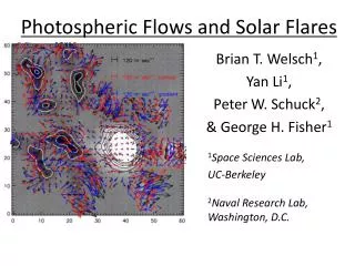
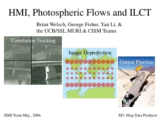
HMI, Photospheric Flows and ILCT . Brian Welsch, George Fisher, Yan Li, & the UCB/SSL MURI & CISM Teams. Correlation Tracking. Image Deprojection. Output Pipeline. HMI Team Mtg., 2006. M3: Mag Data Products.

E N D
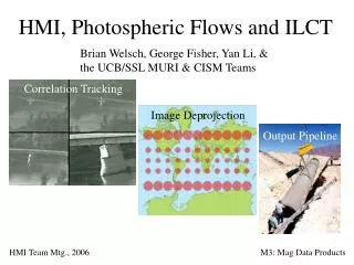
HMI, Photospheric Flows and ILCT Brian Welsch, George Fisher, Yan Li, & the UCB/SSL MURI & CISM Teams Correlation Tracking Image Deprojection Output Pipeline HMI Team Mtg., 2006 M3: Mag Data Products
Velocity inversions generate a 2D map v(x1,x2)from one 2D image, f1(x1,x2), to another, f2(x1,x2). The map depends upon: • the difference f(x1,x2) = f2(x1,x2) – f1(x1,x2) • assumption(s) relating v(x1,x2) to f/t, e.g.: • continuity equation, f/t + t(vtf) = 0, or • advection equation, f/t + (vtt)f = 0, etc. Based on the assumption chosen, v(x1,x2) is not necessarily velocity – e.g., group velocity of interference patterns.
Local correlation tracking (LCT) finds v(x1,x2) by correlating subregions; it assumes advection. = * = = 4) v(xi, yi) is inter- polated max. of correlation funct 1) for ea. (xi, yi) above |B|threshold… 2) apply Gaussian mask at (xi, yi) … 3) truncate and cross-correlate… HMI+AIA, M3: Mag Data Products
Demoulin & Berger (2003) argued that LCT applied to magnetograms does not necessarily give plasma velocities. Motion of flux across photosphere, uf, can be a combination of horizontal & vertical flows acting on non-vertical fields. uf vnBh-vhBn is the flux transport velocity • uf is the apparent velocity (2 components) • v is the actual plasma velocity (3 comps)
The magnetic induction equation’s normal component relates velocities to dBn/dt. Bn/t = h(vnBh-vhBn) = -h(ufBn) • In fact, -h(uLCTBn) only approximatesBn/t, so uLCT uf • Inductive LCT (ILCT) finds uf that matches Bn/t exactly and closely matches uLCT. • Writing ufBn = -h + h x( n), we find • via Bn/t = h2 • by assuming uf = uLCT, so h2 = - h x(uLCTBn) HMI+AIA, M3: Mag Data Products
Aside: fundamentally, two components of uf(x1,x2) cannot determine three components of plasma velocity, v(x1,x2). • Hence, other velocity fields v(x1,x2) consistent with Bn/t can be found. • Other techniques available include: • Minimum Energy Fit (MEF, Longcope, 2004) • Differential LCT (DLCT) & Differential Affine Velocity Estimator (DAVE) (Schuck, 2006) HMI+AIA, M3: Mag Data Products
The FLCT code’s current version combines pro- grams written in IDL & C, and open source code. • IDL • C • Standard C library routines: stdio.h, stdlib.h, math.h • Fastest Fourier Transform in the West (FFTW), v. 3.0 • The executable has been compiled & tested on several architectures. • Linux • Solaris • Windows • Macintosh
Matching HMI’s 10-minute vector magnetogram cadence will be challenging. • HMI has Npix ~ 107 pixels within 60o of disk center. • - MDI’s 10242 HMI’s 40962 x 16 • - MDI, w/in ~30o HMI, w/in ~60o x 2.5 • We track pixels with |Bn| > |B|thresh = 20G • ~ 25% of Npix at solar max. • ~ 5% of Npix at solar min. • FLCT speed is ~linear in Npix correlated. • - t ~ (1 sec/100 pix) x (2.5 x 10⁶ pix) ~ 2.5 x 10⁴ sec ~ 7 hr! • - at solar min., w/ |B|thresh = 100G (~1% of Npix), t ~ 20 min.
Velocity estimates work from difference images, so temporal artifacts must be removed. IVM difference images of BLOS in AR 9026, with a ~4 min. cadence, show large-scale, alternating field fluctuations that inhibit accurate tracking. HMI+AIA, M3: Mag Data Products
Accurate velocity estimates also require deprojection of full-disk magnetograms. • Away from disk center, flows with a component along LOS are foreshortened by curvature of the solar surface. • Conformal deprojections, e.g., Mercator, locally preserve angles; scales are distorted, but easily fixed. • This is optimal for tracking, since neither flow component is biased by the deprojection. • (Apparent changes in lengths perpendicular to the LOS from center-to-limb are negligible.)
FLCT was initially tested using a known image. We found FLCT could accurately reconstruct the imposed flow.
FLCT was also tested on magnetograms with imposed differential rotation – again, recovering the input flow. White dots are imposed differential rotation profile; red dots are raw velocities from Mercator projection; green are properly rescaled; white diamonds are latitudinally binned averages of green dots. HMI+AIA, M3: Mag Data Products
We have implemented a preliminary, automated “Magnetic Evolution Pipeline” (MEP). http://solarmuri.ssl.berkeley.edu/~welsch/public/data/Pipeline/ • cron checks for new magnetograms with wget • New magnetograms are downloaded, deprojected, and tracked using FLCT. • The output stream includes deprojected m-grams, FLCT flows (.png graphics files & ASCII data files), and tracking parameters. • Full documentation & all codes are on line. HMI+AIA, M3: Mag Data Products
Several performance-enhancing modifications to FLCT were implemented and more are planned. • Sub-pixel interpolation was made more efficient. • Correlation is now accomplished by spawning a C subroutine that employs FFTW. • FLCT is readily parallelizable; we envision this “soon.” • Computing velocities in neighborhoods, as opposed to each pixel, is another way to increase speed. HMI+AIA, M3: Mag Data Products
Conclusions • Accurate flow estimates will require • deprojection of full-disk magnetograms, and • careful temporal filtering. • Matching planned data cadences will be challenging. Solutions: • parallelization • find v(x1,x2) on tiles, not every pixel • more restricitve |Bn| thresholding • Essential tools for an LCT pipeline are in place. HMI+AIA, M3: Mag Data Products
References • Démoulin & Berger, 2003: Magnetic Energy and Helicity Fluxes at the Photospheric Level, Démoulin, P., and Berger, M. A. Sol. Phys., v. 215, # 2, p. 203-215. • Longcope, 2004:Inferring a Photospheric Velocity Field from a Sequence of Vector Magnetograms: The Minimum Energy Fit, ApJ, v. 612, # 2, p. 1181-1192. • Schuck, 2005:Tracking Magnetic Footpoints with the Magnetic Induction Equation, ApJ (submitted, 2006) • Welsch et al., 2004:ILCT: Recovering Photospheric Velocities from Magnetograms by Combining the Induction Equation with Local Correlation Tracking, Welsch, B. T., Fisher, G. H., Abbett, W.P., and Regnier, S., ApJ, v. 610, #2, p. 1148-1156. HMI+AIA, M3: Mag Data Products
Yang’s e-mail. • “It would be great if you can talk about your ILCT method/ code • during the session. Because this session is ‘data products’ session, • … briefly summarize your algorithm first, and then focus on • addressing following issues: • Nature of the codes (Language, etc); • Additional supporting software (IDL, MATHLIB, ...); • Computational requirements (run time estimate, system requirements, etc); • Requirements for the input data & format of the output products; • Potential challenges, test procedures, target date for completion of codes, etc... • Time is 15 minutes, but … leave 5 minutes for further discussion.”