Download
1 / 11

E N D
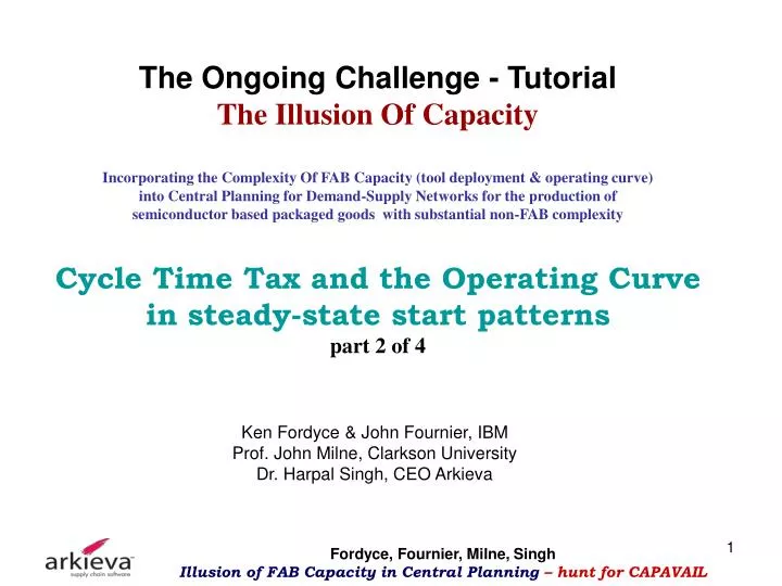
The Ongoing Challenge - TutorialThe Illusion Of CapacityIncorporating the Complexity Of FAB Capacity (tool deployment & operating curve) into Central Planning for Demand-Supply Networks for the production of semiconductor based packaged goods with substantial non-FAB complexityCycle Time Tax and the Operating Curvein steady-state start patternspart 2 of 4 Ken Fordyce & John Fournier, IBMProf. John Milne, Clarkson UniversityDr. Harpal Singh, CEO Arkieva Fordyce, Fournier, Milne, Singh Illusion of FAB Capacity in Central Planning – hunt for CAPAVAIL
Hunt for CAPAVAIL and the Operating Curve Fordyce, Fournier, Milne, Singh Illusion of FAB Capacity in Central Planning – hunt for CAPAVAIL
Outline • Overview of the Demand Supply Network for the production of semiconductor based package goods • Warring factions • Decision Tiers • Aggregate FAB Planning • Central Planning • Two major challenges • Planned lack of tool uniformity • Inherent variability • Basics of Aggregate Factory Planning • Can this wafer start profile be supported • Near Term Deployment • WIP Projection • Basics of Central Planning • Basic Functions • Historical emphasis on non-FAB complexity • Alternate BOM for example • Handle FAB Capacity with limits stated as wafer starts • Wafer start equivalents evolved to nested wafer starts • Second look at capacity (CAPREQ and CAPAVAIL) • Linear methods in central planning engines • FAB complexity creates miss match • Operating Curve and Cycle time Tax Fordyce, Fournier, Milne, Singh Illusion of FAB Capacity in Central Planning – hunt for CAPAVAIL
definitions • CAPREQ - establishing a consumption rate for each unit of production by that manufacturing activity for the selected resource • CAPAVAIL - providing the total available capacity for the resource. connecting manufacturing releases (starts) to resource consumption with a linear relationship Fordyce, Fournier, Milne, Singh Illusion of FAB Capacity in Central Planning – hunt for CAPAVAIL
CAPAVAIL, Cycle Time, & a Taxes • Central & FAB Planning make two demand supply network decisions • quantity of wafer starts (explicit decision made by CPE) • committed cycle time (input to CPE) • Typically cycle time is “fixed” and not linked to starts decision • In fact committed cycle time influences capacity available • Longer cycle times, more effective capacity available • Shorter cycle times, less effective capacity available • since capacity available influences starts, the two decisions (starts and cycle time are not independent • Shorter cycle time, less starts • Longer cycle time more starts • use operating curve to link cycle time and effective capacity available via a cycle time tax Fordyce, Fournier, Milne, Singh Illusion of FAB Capacity in Central Planning – hunt for CAPAVAIL
Trade-off between effective capacity available and cycle time For Blue Operating Curve to achieve a CTM of 5.00 Requires accepting Tool utilization of 80% IDLE IS TAX Which Means 20% of your capacity has to SIT IDLE If you are willing to accept CTM of 6.0, then only 17% of your capacity has to sit idle Effective CAPAVAIL is 80% of “Raw” CAPAVAIL Effective CAPAVAIL is 83% of “Raw” CAPAVAIL Fordyce, Fournier, Milne, Singh Illusion of FAB Capacity in Central Planning – hunt for CAPAVAIL
Martin-Morrison Operating Curve – some basics Cycle Time Estimate Based on Utilization • CTM is the cycle time multiplier of raw process time (RPT) – measure of cycle time • util is tool utilization of the entity (expressed as a percentage) – facility, tool set, checkout clerks, etc. • offset represents several of aspects of the process that generate wait time that cannot be eliminated. • M is the number of identical parallel machines or servers. Typically this value ranges from 1 to 4 • α represents the amount of variation in the system (arrival times, service times (including machine outage, raw process time (RPT), and operator availability)) and controls how long the curve stays flat. The lower the value of α the less variation and the longer the curve stays flat. Fordyce, Fournier, Milne, Singh Illusion of FAB Capacity in Central Planning – hunt for CAPAVAIL
Martin-Morrison Operating Curve – some basics Utilization Required based on Cycle Time Decision Solve Previous Equation for Util Given a CTM target, calculate tool utilization required This drives idle without WIP • Utilization fraction of tool set required to meet cycle time commit Fordyce, Fournier, Milne, Singh Illusion of FAB Capacity in Central Planning – hunt for CAPAVAIL
Capacity Available Tax Rate to meet cycle time commit where util is a function of the cycle time commit and the operating curve for tool set • CAPAVAIL tax rate is required idle without WIP to meet cycle time target • If the cycle time target requires a 80% utilization, then the “tax” is 20% • If the raw CAPAVAIL is 100 units, then 20 units must be “set aside” to meet the cycle time commit • 20% of the time the tool set should be ready to go, but idle no WIP Fordyce, Fournier, Milne, Singh Illusion of FAB Capacity in Central Planning – hunt for CAPAVAIL
Martin-Morrison Operating Curve – some basics Capacity Required Uplift Factor (ULF) to meet cycle time commit • Alternative is to place “tax” on capacity required (CAPREQ) • This is done with uplift factor • If util is 0.80, then the uplift factor is 1.25 (=1/0.8) • If core CAPREQ is 10, CAPREQ to account for required idle capacity is 12.5 = (10 x 1.25) Fordyce, Fournier, Milne, Singh Illusion of FAB Capacity in Central Planning – hunt for CAPAVAIL
Therefore effective Capacity Availabledepends on the cycle time commit • relationship normally not a component of CPE formulations • cycle time “decisions” are made prior to creation of the central plan in “off line” analysis and seen as an “estimate” of capability as much as a decision • in aggregate FAB planning using algebraic methods incorporating cycle time tax is straightforward, but cumbersome • Challenge is to incorporate this into the day to day central planning process where complications abound • example ramp up or ramp down of cycle time Fordyce, Fournier, Milne, Singh Illusion of FAB Capacity in Central Planning – hunt for CAPAVAIL