Download
1 / 40
400 likes | 535 Views
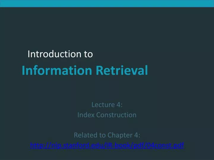
Lecture 4: Index Construction Related to Chapter 4: http://nlp.stanford.edu/IR-book/pdf/04const.pdf. This lecture. Scaling index construction Distributed indexing Dynamic indexing. Sec. 4.2. Inverted index construction.

E N D
Lecture 4: Index Construction Related to Chapter 4: http://nlp.stanford.edu/IR-book/pdf/04const.pdf
This lecture • Scaling index construction • Distributed indexing • Dynamic indexing
Sec. 4.2 Inverted index construction • Documents are parsed to extract words and these are saved with the Document ID. Doc 1 Doc 2 I did enact Julius Caesar I was killed i' the Capitol; Brutus killed me. So let it be with Caesar. The noble Brutus hath told you Caesar was ambitious
Sec. 4.2 After all documents have been parsed, the inverted file is sorted by terms and then by Doc# Key step We focus on this sort step. We have 100M items to sort.
Sec. 4.2 Scaling index construction • In-memory index construction does not scale • Can’t stuff entire collection into memory, sort, then write back • How can we construct an index for very large collections?
Sec. 4.1 Hardware basics • Many design decisions in information retrieval are based on the characteristics of hardware • We begin by reviewing hardware basics
Sec. 4.1 Hardware basics • Access to data in memory is much faster than access to data on disk. • Servers used in IR systems now typically have several GB of main memory, sometimes tens of GB. • Available disk space is several orders of magnitude larger.
Sec. 4.1 Hardware basics • It takes a while for the disk head to move to the part of the disk where the data are located: seek time. • Therefore chunks of data that will be read together should therefore be stored contiguously. • In fact transferring one large chunk of data from disk to memory is faster than transferring many small chunks.
Hardware basics • Disk I/O is block-based: Reading and writing of entire blocks (as opposed to smaller chunks). • Block sizes: 8KB to 256 KB.
Sec. 4.2 RCV1: Our collection for this lecture • Shakespeare’s collected works definitely aren’t large enough for demonstrating many of the points in this course. • As an example for applying scalable index construction algorithms, we will use the Reuters RCV1 collection. • This is one year of Reuters newswire. • It isn’t really large enough either, but it’s publicly available and is at least a more plausible example.
Sec. 4.2 A Reuters RCV1 document
Sec. 4.2 Reuters RCV1 statistics • symbol statistic value • N documents 800,000 • M terms 400,000 • tokens 100,000,000
Sec. 4.2 Sort-based index construction • As we build the index, we parse docs one at a time. • At 12 bytes (4+4+4) per token entry (term, doc, freq), demands a lot of space for large collections. • Why 4 bits per term? • “Term to term-id” dictionary and “term-id to doc-id” dictionary. • T = 100,000,000 in the case of RCV1 • We can do this in memory in 2009, but typical collections are much larger. E.g., the New York Times provides an index of >150 years of newswire • Thus: We need to store intermediate results on disk.
Sec. 4.2 Sort using disk as “memory”? • Can we use the same index construction algorithm for larger collections, but by using disk instead of memory? • Sorting T = 100,000,000 records on disk is too slow • Too many (random) disk seeks.
The solution? • We need to use an external sorting algorithm, that is, one that uses disk. • For acceptable speed, the central requirement of such an algorithm is that it minimize the number of random disk seeks during sorting. • Sequential disk reads are far faster than seeks. • Two methods: • BSBI • SPIMI (not present in our course)
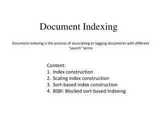
BSBI: Blocked Sort-Based Indexing • (i) segments the collection into parts of equal size, • (ii) sort and invert the termID–docID pairs of each part in memory, • First, we sort the termID–docID pairs. • Next, we collect all termID–docID pairs with the same termID into a postings list • (iii) stores intermediate sorted results on disk, • (iv) merges all intermediate results into the final index.
Sec. 4.2 Example • Must now sort 100M records. • Define a Block ~ 10M such records • Can easily fit a couple into memory. • Will have 10 such blocks to start with.
Sec. 4.2 How to merge the sorted runs?
How to merge the sorted runs? • Open all block files simultaneously. • Maintain small read buffers for the ten blocks and a write buffer for the final merged index we are writing. • In each iteration, we select the lowest termID that has not been processed yet. • All postings lists for this termID are read and merged, and the merged list is written back to disk. • Each read buffer is refilled from its file when necessary.
Sec. 4.2 How to merge the sorted runs? • Providing you read decent-sized chunks of each block into memory and then write out a decent-sized output chunk, then you’re not killed by disk seeks
Sec. 4.3 Remaining problem with sort-based algorithm • Our assumption was: we can keep the dictionary in memory. • We need the dictionary (which grows dynamically) in order to implement a term to termID mapping. • Actually, we could work with term,docID postings instead of termID,docID postings • But then intermediate files become very large. (We would end up with a scalable, but very slow index construction method) • The solution: SPMI method.
This lecture • Scaling index construction • Distributed indexing • Dynamic indexing
An example of distributed processing • 10000$ prize for recognizing the content of a file that are encrypted with DES algorithm. • 96 days later, RockeVerser won this prize with distributed processing. • 70000 computers were used for this purpose. • Each computer tested a small part of the key search space.
Sec. 4.4 Distributed indexing • For web-scale indexing (don’t try this at home!): • must use a distributed computing cluster • a group of tightly coupled computers that work together closely • Individual machines are fault-prone • Can unpredictably slow down or fail • How do we exploit such a pool of machines? • Estimate: Google ~1 million servers, 3 million processors/cores (Gartner 2007)
Sec. 4.4 Distributed indexing • Maintain a mastermachine directing the indexing job • considered “safe”. • Break up indexing into sets of (parallel) tasks. • Master machine assigns each task to an idle machine from a pool.
Sec. 4.4 Parallel tasks • We will use two sets of parallel tasks • Parsers • Inverters • Break the input document collection into splits • Each split is a subset of documents (corresponding to blocks in BSBI/SPIMI)
Sec. 4.4 Parsers • Master assigns a split to an idle parser machine • Parser reads a document at a time and emits (term, doc) pairs • Parser writes pairs into jpartitions • Each partition is for a range of terms’ first letters • (e.g., a-f, g-p, q-z) – here j = 3.
Sec. 4.4 Inverters • An inverter collects all (term,doc) pairs (= postings) for one term-partition. • Sorts and writes to postings lists
Sec. 4.4 Data flow Master assign assign Postings Parser Inverter a-f g-p q-z a-f Parser a-f g-p q-z Inverter g-p Inverter splits q-z Parser a-f g-p q-z Map phase Reduce phase Segment files
Sec. 4.4 MapReduce • The index construction algorithm we just described is an instance of MapReduce. • MapReduce (Dean and Ghemawat 2004) is a robust and conceptually simple framework for distributed computing • without having to write code for the distribution part.
This lecture • Scaling index construction • Distributed indexing • Dynamic indexing
Sec. 4.5 Dynamic indexing • Up to now, we have assumed that collections are static. • They rarely are: • Documents come in over time and need to be inserted. • Documents are deleted and modified. • This means that the dictionary and postings lists have to be modified: • Postings updates for terms already in dictionary • New terms added to dictionary
The simplest approach • Periodically reconstruct the index. • This is a good solution if • The number of changes over time is small • Delay in making new documents searchable is acceptable • Enough resources are available to construct a new index while the old one is still available for querying.
Sec. 4.5 Another approach • Maintain “big” main index • New docs go into “small” auxiliary index • Search across both, merge results • Deletions • Invalidation bit-vector for deleted docs • Filter docs output on a search result by this invalidation bit-vector • Documents are updated by deleting and reinserting them. • Periodically, re-index into one main index.
Merging • Number of merges: times. • is the size of auxiliary index. • is the total number of postings. • Thus, the overall time complexity is • We can do better by logarithmic merge: • Introducing indexes of size
Logarithmic Merging K: the number of times, auxiliary is filled.
Sec. 4.5 Logarithmic merge
Final considerations • So far, postings lists are ordered with respect to docID. • As we see in Chapter 5, this is advantageous for compression. • However, this structure for the index is not optimal when we build ranked retrieval systems(chapter 6 and 7). • In ranked retrieval, postings are often ordered according to weight or impact. • In a docID-sorted index, new documents are always inserted at the end of postings lists. • In an impact-sorted index, the insertion can occur anywhere, thus complicating the update of the inverted index.