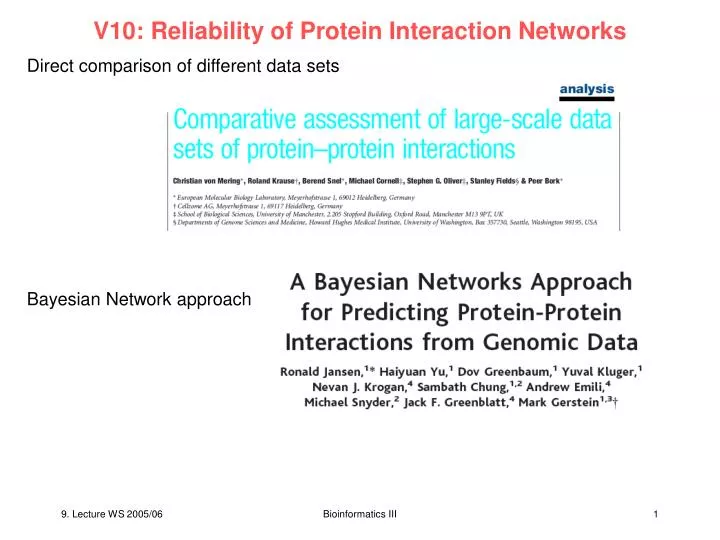
V10: Reliability of Protein Interaction Networks

1. V10: Reliability of Protein Interaction Networks Direct comparison of different data sets Bayesian Network approach Bioinformatics III

2. High-throughput methods for detecting protein interactions Yeast two-hybrid assay. Pairs of proteins to be tested for interaction are expressed as fusion proteins ('hybrids') in yeast: one protein is fused to a DNA-binding domain, the other to a transcriptional activator domain. Any interaction between them is detected by the formation of a functional transcription factor. Benefits: it is an in vivo technique; transient and unstable interactions can be detected; it is independent of endogenous protein expression; and it has fine resolution, enabling interaction mapping within proteins. Drawbacks: only two proteins are tested at a time (no cooperative binding); it takes place in the nucleus, so many proteins are not in their native compartment; and it predicts possible interactions, but is unrelated to the physiological setting. Mass spectrometry of purified complexes. Individual proteins are tagged and used as 'hooks' to biochemically purify whole protein complexes. These are then separated and their components identified by mass spectrometry. Two protocols exist: tandem affinity purification (TAP), and high-throughput mass-spectrometric protein complex identification (HMS-PCI). Benefits: several members of a complex can be tagged, giving an internal check for consistency; and it detects real complexes in physiological settings. Drawbacks: it might miss some complexes that are not present under the given conditions; tagging may disturb complex formation; and loosely associated components may be washed off during purification. Correlated mRNA expression (synexpression). mRNA levels are systematically measured under a variety of different cellular conditions, and genes are grouped if they show a similar transcriptional response to these conditions. These groups are enriched in genes encoding physically interacting proteins. Benefits: it is an in vivo technique, albeit an indirect one; and it has much broader coverage of cellular conditions than other methods. Drawbacks: it is a powerful method for discriminating cell states or disease outcomes, but is a relatively inaccurate predictor of direct physical interaction; and it is very sensitive to parameter choices and clustering methods during analysis. Von Mering et al. Nature 417, 399 (2002) Bioinformatics III

3. High-throughput methods for detecting protein interactions Genetic interactions (synthetic lethality). Two nonessential genes that cause lethality when mutated at the same time form a synthetic lethal interaction. Such genes are often functionally associated and their encoded proteins may also interact physically. This type of genetic interaction is currently being studied in an all-versus-all approach in yeast. Benefits: it is an in vivo technique, albeit an indirect one; and it is amenable to unbiased genome-wide screens. In silico predictions through genome analysis. Whole genomes can be screened for three types of interaction evidence: (1) in prokaryotic genomes, interacting proteins are often encoded by conserved operons; (2) interacting proteins have a tendency to be either present or absent together from fully sequenced genomes, that is, to have a similar 'phylogenetic profile'; and (3) seemingly unrelated proteins are sometimes found fused into one polypeptide chain. This is an indication for a physical interaction. Benefits: fast and inexpensive in silico techniques; and coverage expands as more genomes are sequenced. Drawbacks: it requires a framework for assigning orthology between proteins, failing where orthology relationships are not clear; and so far it has focused mainly on prokaryotes. Von Mering et al. Nature 417, 399 (2002) Bioinformatics III

4. Data set Experiment: Uetz et al. 957 interactions Ito et al. 4549 interactions HMS-PCI 33014 interactions In silico: Conserved gene neighborhood 6387 interactions Gene fusions 358 interactions Co-occurrence of genes 997 interactions Von Mering et al. Nature 417, 399 (2002) Bioinformatics III

5. Counting interactions Various high-throughput methods give differing results on the same complex. >80.000 interactions available for yeast. Only 2.400 are supported by more than 1 method. • Possible explanations ? • Methods may not have reached saturation • Many of the methods produce a significant fraction of false positives • Some methods may have difficulties for certain types of interactions Von Mering et al. Nature 417, 399 (2002) Bioinformatics III

6. Protein interactions between functional categories Each technique produces a unique distribution of interactions with respect to functional categories  methods have specific strengths and weaknesses. E.g. TAP and HMS-PCI predict few interactions for proteins involved in transport and sensing because these categories are enriched with membrane proteins. E.g. Y2H detects few proteins involved in translation. Von Mering et al. Nature 417, 399 (2002) Bioinformatics III

7. Complementarity between data sets • Glycine decarboxylase • Multienzyme complex needed when Gly is used as 1-carbon source. • Its key components GCV1, GCV2, GCV3 are only induced when there is excess Glycine and folate levels are low. This may explain why complex is not detected in experiments. • However, 3 components can be detected by several independent in silico methods • Gene neighborhood of all 3 components in 7 diverged species • genes show very similar phylogenetic distribution • microarrays: genes are closely co-regulated. Opposite example: PPH3 protein Complex found in 4 independent purifications, but no in silico method predicts interaction. Von Mering et al. Nature 417, 399 (2002) Bioinformatics III

8. Quantitative comparison of interaction data sets The various data sets are benchmarked against a reference set of 10,907 trusted interactions, which are derived from protein complexes annotated manually at MIPS and YPD databases. Coverage and accuracy are lower limits owing to incompleteness of the reference set. Each dot in the graph represents an entire interaction data set. For the combined evidence, consider only interactions supported by an agreement of two (or three) of any of the methods shown. Von Mering et al. Nature 417, 399 (2002) Bioinformatics III

9. Biases in interaction coverage Experiment: Uetz et al. 957 interactions Ito et al. 4549 interactions HMS-PCI 33014 interactions In silico: Conserved gene neighborhood 6387 interactions Gene fusions 358 interactions Co-occurrence of genes 997 interactions None of the methods covers more than 60% of the proteins in the yeast genome. Are there common biases as to which proteins are covered? Von Mering et al. Nature 417, 399 (2002) Bioinformatics III

10. Bias 1 towards proteins of high abundance mRNA abundance is a rough measure of protein abundance. Here, divide yeast genome into 10 mRNA abundance classes (bins) of equal size. For each data set and abundance class, the number of interactions is recorded having at least one protein in that class. Each interaction (A–B) is counted twice: once under the abundance class of partner A, and once under the abundance class of partner B.  Most data sets are heavily biased towards proteins of high abundance except for genetic techniques (Y2H and synthetic lethality) Von Mering et al. Nature 417, 399 (2002) Bioinformatics III

11. Bias 2 towards cellular localization Protein localization and interaction coverage. Protein localizations are derived from the MIPS and TRIPLES databases. a, The distribution of protein localization among the proteins covered by a data set. E.g. in silico predictions overestimate mitochondrial interactions. Von Mering et al. Nature 417, 399 (2002) Bioinformatics III

12. Bias 2 towards cellular localization Independent quality measure: Are proteins that interact belong to the same compartment? Y2H method gives relatively poor results here. Von Mering et al. Nature 417, 399 (2002) Bioinformatics III

13. Bias 3 in interaction coverage Separate yeast genome into 4 classes according to the conservation of the genes in other species The presence of a gene in any of these species was concluded from bi-directional best hits in Swiss-Waterman searches, using 0.01 as cut-off. Bias related to the degree of evolutionary novelty of proteins. Proteins restricted to yeast are less well covered than ancient, evolutionarily conserved proteins. Von Mering et al. Nature 417, 399 (2002) Bioinformatics III

14. Outlook • How many protein-protein interactions can be expected in yeast? • Overlap of high-throughput data is 20 times larger than expected by chance. • Good signal-to-noise ratio. Also, for interactions discovered ≥ 2 times, usually both partners have the same functional category and cellular localization. •  Overlap mainly consists of „true positives“. • Less than 1/3 of new interactions in overlap set were previously known. • Given 10.000 currently known interactions predict >30.000 protein interactions in yeast (lower boundary). Von Mering et al. Nature 417, 399 (2002) Bioinformatics III

15. Problems Unfortunately, interaction data sets are often incomplete and contradictory (von Mering et al. 2002). In the context of genome-wide analyses, these inaccuracies are greatly magnified because the protein pairs that do not interact (negatives) by far outnumber those that do interact (positives). E.g. in yeast, the ~6000 proteins allow for N (N-1) / 2 ~ 18 million potential interactions. But the estimated number of actual interactions is < 100.000. Therefore, even reliable techniques can generate many false positives when applied genome-wide. Think of a diagnostic with a 1% false-positive rate for a rare disease occurring in 0.1% of the population. This would roughly produce 1 true positive for every 10 false ones. Jansen et al. Science 302, 449 (2003) Bioinformatics III

16. Integrative Approach One would like to integrate evidence from many different sources to increase the predictivity of true and false protein-protein predictions. Here, use Bayesian approach for integrating interaction information that allows for the probabilistic combination of multiple data sets; apply to yeast. Input: Approach can be used for combining noisy genomic interaction data sets. Normalization: Each source of evidence for interactions is compared against samples of known positives and negatives (“gold-standard”). Output: predict for every possible protein pair likelihood of interaction. Verification: test on experimental interaction data not included in the gold-standard + new TAP (tandem affinity purification experiments). Jansen et al. Science 302, 449 (2003) Bioinformatics III

17. Integration of various information sources 3 different types of data used: (i) Interaction data from high-throughput experiments. These comprise large-scale two-hybrid screens (Y2H) and in vivo pull-down experiments. (ii) Other genomic features: expression data, biological function of proteins (from Gene Ontology biological process and the MIPS functional catalog), and data about whether proteins are essential. (iii) Gold-standards of known interactions and noninteracting protein pairs. Jansen et al. Science 302, 449 (2003) Bioinformatics III

18. Combination of data sets into probabilistic interactomes The 4 interaction data sets from HT experiments were combined into 1 PIE. The PIE represents a transformation of the individual binary-valued interaction sets into a data set where every protein pair is weighed according to the likelihood that it exists in a complex. (B) Combination of data sets into probabilistic interactomes. A „naïve” Bayesian network is used to model the PIP data. These information sets hardly overlap. Because the 4 experimental interaction data sets contain correlated evidence, a fully connected Bayesian network is used. Jansen et al. Science 302, 449 (2003) Bioinformatics III

19. Bayesian Networks Bayesian networks are probabilistic models that graphically encode probabilistic dependencies between random variables. Y A directed arc between variables Y and E1 denotes conditional dependency of E1 on Y, as determined by the direction of the arc. E1 E3 E2 Bayesian networks also include a quantitative measure of dependency. For each variable and its parents this measure is defined using a conditional probability function or a table. Here, one such measure is the probability Pr(E1|Y). Bioinformatics III

20. Bayesian Networks Together, the graphical structure and the conditional probability functions/tables completely specify a Bayesian network probabilistic model. Y This model, in turn, specifies a particular factorization of the joint probability distribution function over the variables in the networks. E1 E3 E2 Here, Pr(Y,E1,E2,E3) = Pr(E1|Y) Pr(E2|Y) Pr(E3|Y) Pr(Y) Bioinformatics III

21. Gold-Standard should be (i) independent from the data sources serving as evidence (ii) sufficiently large for reliable statistics (iii) free of systematic bias (e.g. towards certain types of interactions). Positives: use MIPS (Munich Information Center for Protein Sequences, HW Mewes) complexes catalog: hand-curated list of complexes (8250 protein pairs that are within the same complex) from biomedical literature. Negatives: - harder to define - essential for successful training Assume that proteins in different compartments do not interact. Synthesize “negatives” from lists of proteins in separate subcellular compartments. Jansen et al. Science 302, 449 (2003) Bioinformatics III

22. Measure of reliability: likelihood ratio Consider a genomic feature f expressed in binary terms (i.e. „absent“ or „present“). Likelihood ratio L(f) is defined as: L(f) = 1 means that the feature has no predictability: the same number of positives and negatives have feature f. The larger L(f) the better its predictability. Jansen et al. Science 302, 449 (2003) Bioinformatics III

23. Combination of features For two features f1and f2 with uncorrelated evidence, the likelihood ratio of the combined evidence is simply the product: L(f1,f2) = L(f1)  L(f2) For correlated evidence L(f1,f2) cannot be factorized in this way. Bayesian networks are a formal representation of such relationships between features. The combined likelihood ratio is proportional to the estimated odds that two proteins are in the same complex, given multiple sources of information. Jansen et al. Science 302, 449 (2003) Bioinformatics III

24. Prior and posterior odds „positive“ : a pair of proteins that are in the same complex. Given the number of positives among the total number of protein pairs, the „prior“ odds of finding a positive are: „posterior“ odds: odds of finding a positive after considering N datasets with values f1 ... fN : The terms „prior“ and „posterior“ refer to the situation before and after knowing the information in the N datasets. Jansen et al. Science 302, 449 (2003) Bioinformatics III

25. Static naive Bayesian Networks In the case of protein-protein interaction data, the posterior odds describe the odds of having a protein-protein interaction given that we have the information from the N experiments, whereas the prior odds are related to the chance of randomly finding a protein-protein interaction when no experimental data is known. If Opost> 1, the chances of having an interaction are higher than having no interaction. Jansen et al. Science 302, 449 (2003) Bioinformatics III

26. Static naive Bayesian Networks The likelihood ratio L defined as relates prior and posterior odds according to Bayes‘ rule: In the special case that the N features are conditionally independent (i.e. they provide uncorrelated evidence) the Bayesian network is a so-called „naïve” network, and L can be simplified to: Jansen et al. Science 302, 449 (2003) Bioinformatics III

27. Computation of prior and posterior odds L can be computed from contingency tables relating positive and negative examples with the N features (by binning the feature values f1 ... fNinto discrete intervals) – wait for examples. Determining the prior odds Oprioris somewhat arbitrary in that it requires an assumption about the number of positives. Jansen et al. believe that 30,000 is a conservative lower bound for the number of positives (i.e. pairs of proteins that are in the same complex). Considering that there are ca. 18 million = 0.5 * N (N – 1) possible protein pairs in total (with N = 6000 for yeast), Opost > 1 can be achieved with L > 600. Jansen et al. Science 302, 449 (2003) Bioinformatics III

28. Essentiality (PIP) Consider whether proteins are essential or non-essential = does a deletion mutant where this protein is knocked out from the genome have the same phenotype? It should be more likely that both of 2 proteins in a complex are essential or non-essential, but not a mixture of these two attributes. Deletion mutants of either one protein should impair the function of the same complex. Jansen et al. Science 302, 449 (2003) Bioinformatics III

29. Parameters of the naïve Bayesian Networks (PIP) Column 1 describes the genomic feature. In the „essentiality data“ protein pairs can take on 3 discrete values (EE: both essential; NN: both non-essential; NE: one essential and one not). Column 2 gives the number of protein pairs with a particular feature (i.e. „EE“) drawn from the whole yeast interactome (~18M pairs). Columns „pos“ and „neg“ give the overlap of these pairs with the 8,250 gold-standard positives and the 2,708,746 gold-standard negatives. Columns „sum(pos)“ and „sum(neg)“ show how many gold-standard positives (negatives) are among the protein pairs with likelihood ratio  L, computed by summing up the values in the „pos“ (or „neg“) column. P(feature value|pos) and P(feature value|neg) give the conditional probabilities of the feature values – and L, the ratio of these two conditional probabilities. Jansen et al. Science 302, 449 (2003) Bioinformatics III

30. mRNA expression data Proteins in the same complex tend to have correlated expression profiles. Although large differences can exist between the mRNA and protein abundance, protein abundance can be indirectly and quite crudely measured by the presence or absence of the corresponding mRNA transcript. Experimental data source: - time course of expression fluctuations during the yeast cell cycle - Rosetta compendium: expression profiles of 300 deletion mutants and cells under chemical treatments. Problem: both data sets are strongly correlated. Compute first principal component of the vector of the 2 correlations. Use this as independent source of evidence for the P-P interaction prediction. The first principal component is a stronger predictor of P-P interactions that either of the 2 expression correlation datasets by themselves. Jansen et al. Science 302, 449 (2003) Bioinformatics III

31. mRNA expression data The values for mRNA expression correlation (first principal component) range on a continuous scale from -1.0 to +1.0 (fully anticorrelated to fully correlated). This range was binned into 19 intervals. Jansen et al. Science 302, 449 (2003) Bioinformatics III

32. PIP – Functional similarity Quantify functional similarity between two proteins: - consider which set of functional classes two proteins share, given either the MIPS or Gene Ontology (GO) classification system. - Then count how many of the ~18 million protein pairs in yeast share the exact same functional classes as well (yielding integer counts between 1 and ~ 18 million). It was binned into 5 intervals. - In general, the smaller this count, the more similar and specific is the functional description of the two proteins. Jansen et al. Science 302, 449 (2003) Bioinformatics III

33. PIP – Functional similarity Observation: low counts correlate with a higher chance of two proteins being in the same complex. But signal (L) is quite weak. Jansen et al. Science 302, 449 (2003) Bioinformatics III

34. Calculation of the fully connected Bayesian network (PIE) The 3 binary experimental interaction datasets can be combined in at most 24 = 16 different ways (subsets). For each of these 16 subsets, one can compute a likelihood ratio from the overlap with the gold-standard positives („pos“) and negatives („neg“). Jansen et al. Science 302, 449 (2003) Bioinformatics III

35. Distribution of likelihood ratios Number of protein pairs in the individual datasets and the probabilistic interactomes as a function of the likelihood ratio. There are many more protein pairs with high likelihood ratios in the probabilistic interactomes (PIE) than in the individual datasets G,H,U,I. Protein pairs with high likelihood ratios provide leads for further experimental investigation of proteins that potentially form complexes. Jansen et al. Science 302, 449 (2003) Bioinformatics III

36. Overview PIP and PIE are separately tested against the gold-standard. Jansen et al. Science 302, 449 (2003) Bioinformatics III

37. PIP vs. the information sources Ratio of true to false positives (TP/FP) increases monotonically with Lcut, confirming L as an appropriate measure of the odds of a real interaction. The ratio is computed as: Protein pairs with Lcut > 600 have a > 50% chance of being in the same complex. Jansen et al. Science 302, 449 (2003) Bioinformatics III

38. PIE vs. the information sources 9897 interactions are predicted from PIP and 163 from PIE. In contrast, likelihood ratios derived from single genomic factors (e.g. mRNA coexpression) or from individual interaction experiments (e.g. the Ho data set) did no exceed the cutoff when used alone. This demonstrates that information sources that, taken alone, are only weak predictors of interactions can yield reliable predictions when combined. Jansen et al. Science 302, 449 (2003) Bioinformatics III

39. parts of PIP graph Test whether the thresholded PIP was biased toward certain complexes, compare distribution of predictions among gold-standard positives. (A ) The complete set of gold-standard positives and their overlap with the PIP. The PIP (green) covers 27% of the gold-standard positives (yellow). The predicted complexes are roughly equally apportitioned among the different complexes  no bias. Jansen et al. Science 302, 449 (2003) Bioinformatics III

40. parts of PIP graph Graph of the largest complexes in PIP, i.e. only those proteins having  20 links. (Left) overlapping gold-standard positives are shown in green, PIE links in blue, and overlaps with both PIE and gold-standard positives in black. (Right) Overlapping gold-standard negatives are shown in red. Regions with many red links indicate potential false-positive predictions. Jansen et al. Science 302, 449 (2003) Bioinformatics III

41. experimental verification conduct TAP-tagging experiments (Cellzome) for 98 proteins. These produced 424 experimental interactions overlapping with the PIP threshold at Lcut = 300. Of these, 185 overlapped with gold-standard positives and 16 with negatives. Jansen et al. Science 302, 449 (2003) Bioinformatics III

42. Concentrate on large complexes Sofar all interactions were treated as independent. However, the joint distribution of interactions in the PIs can help identify large complexes: an ideal complex should be a fully connected „clique“ in an interaction graph. In practice, this rarely happens because of incorrect or missing links. Yet large complexes tend to have many interconnections between them, whereas false-positive links to outside proteins tend to occur randomly, without a coherent pattern. Jansen et al. Science 302, 449 (2003) Bioinformatics III

43. Improve ratio TP / FP TP/FP for subsets of the thresholded PIP that only include proteins with a minimum number of links. Requiring a minimum number of links isolates large complexes in the thresholded PIP graph (Fig. 3B). Observation: Increasing the minimum number of links raises TP/FP by preserving the interactions among proteins in large complexes, while filtering out false-positive interactions with heterogeneous groups of proteins outside the complexes. Jansen et al. Science 302, 449 (2003) Bioinformatics III

44. Summary Bayesian approach allows reliable predictions of protein-protein interactions by combining weakly predictive genomic features. The de novo prediction of complexes replicated interactions found in the gold-standard positives and PIE. Also, several predictions were confirmed by new TAP experiments. The accuracy of the PIP was comparable to that of the PIE while simultaneously achieving greater coverage. In a similar manner, the approach could have been extended to a number of other features related to interactions (e.g. phylogenetic co-occurrence, gene fusions, gene neighborhood). As a word of caution: Bayesian approaches don‘t work everywhere. Jansen et al. Science 302, 449 (2003) Bioinformatics III