Download
1 / 23
300 likes | 682 Views
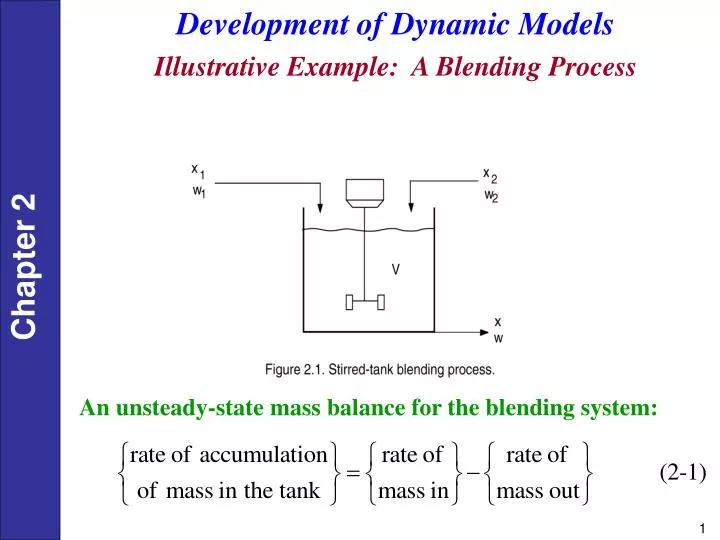
Development of Dynamic Models Illustrative Example: A Blending Process. An unsteady-state mass balance for the blending system:. or where w 1 , w 2 , and w are mass flow rates. The unsteady-state component balance is:.

E N D
Development of Dynamic Models • Illustrative Example: A Blending Process An unsteady-state mass balance for the blending system:
or where w1, w2, and w are mass flow rates. • The unsteady-state component balance is: The corresponding steady-state model was derived in Ch. 1 (cf. Eqs. 1-1 and 1-2).
General Modeling Principles • The model equations are at best an approximation to the real process. • Adage: “All models are wrong, but some are useful.” • Modeling inherently involves a compromise between model accuracy and complexity on one hand, and the cost and effort required to develop the model, on the other hand. • Process modeling is both an art and a science. Creativity is required to make simplifying assumptions that result in an appropriate model. • Dynamic models of chemical processes consist of ordinary differential equations (ODE) and/or partial differential equations (PDE), plus related algebraic equations.
Table 2.1. A Systematic Approach for Developing Dynamic Models • State the modeling objectives and the end use of the model. They determine the required levels of model detail and model accuracy. • Draw a schematic diagram of the process and label all process variables. • List all of the assumptions that are involved in developing the model. Try for parsimony; the model should be no more complicated than necessary to meet the modeling objectives. • Determine whether spatial variations of process variables are important. If so, a partial differential equation model will be required. • Write appropriate conservation equations (mass, component, energy, and so forth).
Table 2.1. (continued) • Introduce equilibrium relations and other algebraic equations (from thermodynamics, transport phenomena, chemical kinetics, equipment geometry, etc.). • Perform a degrees of freedom analysis (Section 2.3) to ensure that the model equations can be solved. • Simplify the model. It is often possible to arrange the equations so that the dependent variables (outputs) appear on the left side and the independent variables (inputs) appear on the right side. This model form is convenient for computer simulation and subsequent analysis. • Classify inputs as disturbance variables or as manipulated variables.
Table 2.2. Degrees of Freedom Analysis • List all quantities in the model that are known constants (or parameters that can be specified) on the basis of equipment dimensions, known physical properties, etc. • Determine the number of equations NE and the number of process variables, NV. Note that time t is not considered to be a process variable because it is neither a process input nor a process output. • Calculate the number of degrees of freedom, NF = NV - NE. • Identify the NE output variables that will be obtained by solving the process model. • Identify the NF input variables that must be specified as either disturbance variables or manipulated variables, in order to utilize the NF degrees of freedom.
Theoretical models of chemical processes are based on conservation laws. • Conservation Laws Conservation of Mass Conservation of Component i
Conservation of Energy The general law of energy conservation is also called the First Law of Thermodynamics. It can be expressed as: The total energy of a thermodynamic system, Utot, is the sum of its internal energy, kinetic energy, and potential energy:
For the processes and examples considered in this book, it • is appropriate to make two assumptions: • Changes in potential energy and kinetic energy can be neglected because they are small in comparison with changes in internal energy. • The net rate of work can be neglected because it is small compared to the rates of heat transfer and convection. • For these reasonable assumptions, the energy balance in • Eq. 2-8 can be written as
The analogous equation for molar quantities is, where is the enthalpy per mole and is the molar flow rate. In order to derive dynamic models of processes from the general energy balances in Eqs. 2-10 and 2-11, expressions for Uint and or are required, which can be derived from thermodynamics. The Blending Process Revisited For constant , Eqs. 2-2 and 2-3 become:
Equation 2-13 can be simplified by expanding the accumulation term using the “chain rule” for differentiation of a product: Substitution of (2-14) into (2-13) gives: Substitution of the mass balance in (2-12) for in (2-15) gives: After canceling common terms and rearranging (2-12) and (2-16), a more convenient model form is obtained:
Stirred-Tank Heating Process Figure 2.3 Stirred-tank heating process with constant holdup, V.
Stirred-Tank Heating Process (cont’d.) • Assumptions: • Perfect mixing; thus, the exit temperature T is also the temperature of the tank contents. • The liquid holdup V is constant because the inlet and outlet flow rates are equal. • The density and heat capacity C of the liquid are assumed to be constant. Thus, their temperature dependence is neglected. • Heat losses are negligible.
Model Development - I For a pure liquid at low or moderate pressures, the internal energy is approximately equal to the enthalpy, Uint , and H depends only on temperature. Consequently, in the subsequent development, we assume that Uint = H and where the caret (^) means per unit mass. As shown in Appendix B, a differential change in temperature, dT, produces a corresponding change in the internal energy per unit mass, where C is the constant pressure heat capacity (assumed to be constant). The total internal energy of the liquid in the tank is:
Model Development - II An expression for the rate of internal energy accumulation can be derived from Eqs. (2-29) and (2-30): Note that this term appears in the general energy balance of Eq. 2-10. Suppose that the liquid in the tank is at a temperature T and has an enthalpy, . Integrating Eq. 2-29 from a reference temperature Tref to T gives, where is the value of at Tref. Without loss of generality, we assume that (see Appendix B). Thus, (2-32) can be written as:
Model Development - III For the inlet stream Substituting (2-33) and (2-34) into the convection term of (2-10) gives: Finally, substitution of (2-31) and (2-35) into (2-10)
Degrees of Freedom Analysis for the Stirred-Tank Model: 3 parameters: 4 variables: 1 equation: Eq. 2-36 Thus the degrees of freedom are NF = 4 – 1 = 3. The process variables are classified as: 1 output variable: T 3 input variables: Ti, w, Q For temperature control purposes, it is reasonable to classify the three inputs as: 2 disturbance variables: Ti, w 1 manipulated variable: Q
Biological Reactions • Biological reactions that involve micro-organisms and enzyme catalysts are pervasive and play a crucial role in the natural world. • Without such bioreactions, plant and animal life, as we know it, simply could not exist. • Bioreactions also provide the basis for production of a wide variety of pharmaceuticals and healthcare and food products. • Important industrial processes that involve bioreactions include fermentation and wastewater treatment. • Chemical engineers are heavily involved with biochemical and biomedical processes.
Chapter 2 Bioreactions • Are typically performed in a batch or fed-batch reactor. • Fed-batch is a synonym for semi-batch. • Fed-batch reactors are widely used in the pharmaceutical and other process industries. • Bioreactions: • Yield Coefficients:
Fed-Batch Bioreactor Monod Equation Specific Growth Rate Figure 2.11. Fed-batch reactor for a bioreaction.
The exponential cell growth stage is of interest. • The fed-batch reactor is perfectly mixed. • Heat effects are small so that isothermal reactor operation can be assumed. • The liquid density is constant. • The broth in the bioreactor consists of liquid plus solid material, the mass of cells. This heterogenous mixture can be approximated as a homogenous liquid. • The rate of cell growth rg is given by the Monod equation in (2-93) and (2-94). • Modeling Assumptions
Modeling Assumptions (continued) • The rate of product formation per unit volume rp can be expressed as where the product yield coefficientYP/X is defined as: • The feed stream is sterile and thus contains no cells. • General Form of Each Balance
Individual Component Balances • Cells: • Product: • Substrate: • Overall Mass Balance • Mass: