Download
1 / 38

E N D
Data WarehousingTarleton state universityMath 586Instructors: keithemmert, Sean perry, AND Micha Robersoncourse materials: oracle SQL By Example, 4th Edition by Alice RischerTSoftware: Oracle 11GTextbook resource website:http://www.oraclesqlbyexample.com/course Objectives:Understand and apply fundamental SQL functions, expressions, commands etc.A. Create/drop tables/databaseB. Query tablESC. Use aggregate functionsD. USE INNER/OUTER/LEFT/RIGHT JOINSE. Write queries with STRING, NUMERIC, CONVERSION, and date/time functions. CONDUCT QA and integrity checks.
Chapter 1 SQL and data • SQL(pronounced “sequel”)-Structured Query Language • Syntax extensions were added by individual vendors and made their way into… • ANSI(American National Standards Institute) SQL, the standard relational databases used today. • SQL is used by most commercial database applications. No viable alt. language. • Evolves, but basic functionality remains unchanged.
Introduction to databases • A database is an organized collection of data. • A database management system (DBMS) is software that allows the creation, retrieval, and manipulation of data. • A relational database management system (RDBMS) provides this functionality within the context of the relational database theory and the rules defined by Codd.
Lab 1.1—The Relational database • Data is all around; you make use of it every day. When registering for a class, interacting with an ATM, etc.. • Data independence, a user does not need to know on which hard drive and file a particular piece of information is stored. • This provides data consistency and data integrity. • A relational database stores data in tables, essentially a two-dimensional matrix consisting of columns and rows.
Tables • Generally contains data about a single subject • Each table has a unique name that signifies the contents of the data • A database consists of many tables.
Columns • Columns in a table organize the data further. • A table consists of at least one column. • Each column represents a single, low-level detail about a set of data • The name of each column is unique within a table and identifies the data you find in that column
Rows • Each row usually represents one unique set of data within a table. • All of the columns of the rows represent respective data for the row. • Each intersection of a column and row in a table represents a value. ROW Column
NULLS • No value is said to be NULL. • Blanks are not nulls. • Nulls cannot be compared or evaluated because they are unknowns. • null is not greater or less than null • null ≠null
Primary key • Need to uniquely identify data within a table. • You find there is one and only one row in the table by looking for the primary key value. • A system-generated sequence number is called a synthetic or surrogate key. • Best to avoid any primary key that is subject to change. • Only one primary key per table. • More than one column in the primary key is called a composite or concatenated primary key
Foreign Keys • Rather than store rows with repetitive data, the table can be normalized to remove duplications. • A foreign key is where primary key column(s) in a table links to a column(s) in another table which provides more detail information for the original table.
Overview • Within the SQL language there are individual sublanguages • Data Manipulation Language(DML) commands allow you to query, insert, update, and delete data. • Data Definition Language(DDL) allows you to create new database structures such as tables and modify existing ones. • Data Control Language(DCL) allows you to control access to the data.
Lab 1.1 Exercises • Go to page 8 in book • Answer and discuss answers in class.
LAB 1.2 Data Normalization and table Relationships • Eliminates redundancy in tables, avoiding future data manipulation problems. • There are several different rules for minimizing duplication of data, called normal forms. • There are many different normalization rules but the five normal forms and the Boyce-Codd normal form(BCNF) are the most accepted.
First Normal Form • All repeating groups must be removed and placed in a new table. • This design provides more flexibility with the data and less overhead. • Minimizes the need to create multiple rows for one unique identifier.
Second normal form • Uses the First Normal Form rules and… • All the nonkey columns must depend on the entire primary key. • Applies only to composite primary keys.
Third normal form • Uses the Second Normal Form rules and… • Every nonkey column must be a fact about the primary key. • If an attribute depends on a nonkey column then that attribute needs to be moved a different table.
Second normal form (2NF)Third normal form (3NF) 2NF & 3NF Book-Author table shows the violation of the second normal form This table shows the violation of the third normal form The Book & the Publisher tables in the 3rd normal form
Fourth, Fifth, and Boyce-Codd • BCNF is an elaborate version of third normal form and deals with deletion anomalies. • Fourth Normal Form tackles potential problems when three or more columns are part of the unique identifier and their dependencies to each other. • Fifth Normal Form splits the tables even further apart to eliminate all redundancy.
Table relationships • When two tables have common column(s), they are said to have a relationship. The cardinality of a relationship is the actual number of occurrences between them. • (1:M) One-to-many relationship: The most common relationship. The shared column(s) of one table links to many rows in the other. • (1:1) One-to-one relationship: The shared column(s) are unique in each table. • (M:M) Many-to-many relationship: The shared column(s) of each table have multiple rows for each unique value. • Following the rules of relational database, an associative table or intersection table resolves the M:M problem.
Database Schema diagrams • Database schema diagrams are used to graphically depict the relationship between tables. • A “crow’s foot” on one end represents the 1:M relationship.
Cardinality and optionality • The cardinality expresses the ratio of a parent and child table from the perspective of the parent table. It describes how many rows you may find between the two tables for a given primary key value. • The optionality of a relationship is whether or not a row is required (mandatory or optional). It shows whether one row in a table can exist without a row in the related table.
Identifying and nonidentifying relationships • In an identifying relationship, the primary key is propagated to the child entity as part of the primary key. • In a nonidentifying relationship, the foreign key becomes one of the nonkey columns. Nulls are accepted in the foreign key column. • Round edges on a diagram mean the relationship is identifying. Sharp edges mean nonidentifying.
Database development context • Requirements Analysis—Gather data requirements that identify the needs and wants of the users. One of the outputs of his phase is a list of individual data elements that need to be stored. • Conceptual Data Model—Groups the major data elements from the requirements analysis into individual entities with each individual data element referred to as an attribute. Unique identifiers or candidate keys that uniquely distinguish each row are determined. Noncritical attributes are not included in the model.
Database development context Cont. • Logical Data Model—Shows that all the entities, their respective attributes, and the relationship between entities represent the business requirements, without considering the technical issues. Descriptive names and documentation is required. The complete model is called the logical data model, or entity relationship diagram (ERD). In the end, entities are fully normalized, the unique identifier for reach entity is determined, and any many-to-many relationships are resolved into associative entities. • Physical Data Model—Also referred to as the database schema diagram is a graphical model of the physical design implementation of the database. There may be many physical models to choose from. This model uses different terminology. Tables instead of entities, columns instead of attributes, etc..
Transfer from logical to physical model • Entities are resolved to physical tables. • Attributes become columns with specific data types and formats. • Data integrity and consistency are created and physical storage parameters for individual tables are determined. • Indexes are designed. They are database objects that facilitate speedy access to data with the help of a specific column(s) of a table. Indices enhance query performance but they also create overhead when performing deletes/inserts/updates.
denormalization • The act of adding redundancy to the physical database design. • Data designers or architects sometimes purposely add redundancy to their design to increased query performance. • In some application where massive amounts of detailed data are stored and summarized, denormalization is required. • Data warehouse applications are database applications that benefit users who need to analyze large data sets from various angles and use this data for reporting and decision-making purposes. • The primary purpose of a data warehouse is to query, report, and analyze data. Therefore, redundancy is encouraged and necessary for queries to perform efficiently.
Lab 1.2: Exercises • Go to page 27 in book • Answer and discuss answers in class.
Lab 1.3: The Student schema diaggram • Throughout this book and the course the database for a school’s computer education program is sued as a case study on which most exercises are based. • It is important to familiarize yourself with the STUDENT case study diagram. • The STUDENT table contains data about each individual student, such as his or her name, address, employer, and the date the student registered in the program.
The student schema cont. • Data Types are found next to each column name in the diagram. Each column can contain a different type of data. Some of the possible data types are as follows:
The student schema cont. 2 • The COURSE table lists all the available courses that a student may take. The table consists of a PREREQUISITE, a COURSE_NO, a DESCRIPTION, and a COST column. COURSE_NO is the key. • The COURSE table represents a recursive or self-referencing relationship. • A recursive relationship means a column within a table references another column within the same table. • In the COURSE table, the PREREQUISITE column shows which course_no is needed to be completed before the current course_no can be taken. • Nulls are allowed here because the relationship is optional.
The student schema cont. 3 • The SECTION table includes all the individual sections a course may have. An individual course may have zero, one, or many sections, each of which can be taught in different rooms, at different times, and by different instructors. SECTION_ID is the primary key of the table. COURSE_NO is a foreign key. STATE_DATE_TIME shows the date and time the section meets, LOCATION lists the classroom, and CAPACITY shows the maximum number of students that may enroll. • A natural key is a set of column(s) that naturally uniquely identify a row. A computer generated sequence number, called a surrogate key, can be used as a substitute of the natural key..
The student schema cont. 4 • The INSTRUCTOR_ID column is another foreign key column in the SECTION table, linking to the INSTRUCTOR table. • An INSTRUCTOR must always be assigned to a SECTION. It can never be null. But an INSTRUCTOR doesn’t have to teach a class. • A COURSE may have zero, one, or multiple sections. • The INSTRUCTOR table lists information related to an individual instructor, such as name, address, phone, and zip code. The primary key is INSTRUCTOR_ID. The ZIP column is the foreign key column to the ZIPCODE table.
The student schema cont. 5 • Referential integrity does not allow deletion of a primary key value in a parent table that exists in a child as a foreign key table. This would create orphan rows in the child table. • The ENROLLMENT table is an intersection table between the STUDENT and the SECTION table, listing the students enrolled in the various section. It has a composite primary key of STUDENT_ID and SECTION_ID. ENROLL_DATE contains the date the student registered and FINAL_GRADE lists the student’s final grade. A STUDENT may be enrolled in zero, one, or many sections.
The student schema cont. 6 • The GRADE_TYPE table is a lookup table for other tables as it relate to grade information. GRADE_TYPE_CODE in the primary key and lists the unique category of grade. DESCRIPTION describes the abbreviated code. • The GRADE table lists all the grades related to the section in which a student is enrolled. GRADE_CODE_OCCURENCE is a sequence number listing the order of the grade, while NUMERIC_GRADE lists actual grade value. GRADE_CONVERSION in the numeric grade converted to a letter. The primary key columns are STUDENT_ID, SECTION_ID, GRADE_TYPE_CODE, and GRADE_CODE_OCCURENCE.
The student schema cont. 7 • The GRADE_TYPE_WEIGHT table aids in computation of the final grade a student receives for an individual section. Different sections can have finals computed differently. The final grade is determined by using the individual grades of the student and section in the GRADE table in conjunction with this table. The primary key consists of the SECTION_ID and GRADE_TYPE_CODE columns. A GRADE_TYPE_CODE can exist zero, one, or many times.
Lab 1.3: Exercises • Go to page 41 in book • Answer and discuss answers in class.
Chapter 1 complete! • Quiz will be given at the beginning of our next class