Download
1 / 28
280 likes | 286 Views
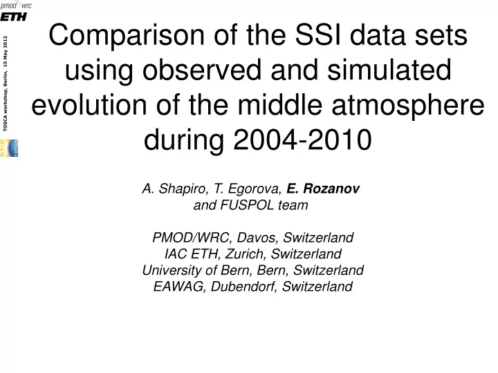
Comparison of the SSI data sets using observed and simulated evolution of the middle atmosphere during 2004-2010. A. Shapiro, T. Egorova, E. Rozanov and FUSPOL team PMOD/WRC, Davos, Switzerland IAC ETH, Zurich, Switzerland University of Bern, Bern, Switzerland EAWAG, Dubendorf, Switzerland.

E N D
Comparison of the SSI data sets using observed and simulated evolution of the middle atmosphere during 2004-2010 A. Shapiro, T. Egorova, E. Rozanov and FUSPOL team PMOD/WRC, Davos, Switzerland IAC ETH, Zurich, Switzerland University of Bern, Bern, Switzerland EAWAG, Dubendorf, Switzerland
Questions • Can we decide which SSI data set is right comparing simulated and measured ozone and temperature time series? • How important is SSI for the future climate warming and ozone recovery?
SSI data sets SORCE data LEAN data 1950 2004.05 2009.02 SIM SOLSTICE LEAN 2007-2004
Key photochemical processes dO3 (‰/nm): Ozone mixing ratio changes due to the observed variability of the spectral solar irradiance (min to max)(Rozanov et al. 2002)
ΔO3 (%) 2004 - 2007 1D-RCPM
CCM SOCOL Lean data 2004.05-2009.02 SIM and SOLSTICE dominated composites 2004.05-2009.02
121 nm 210 nm 290 nm 750 nm CCM SOCOL runs LEAN data + 2 composites: SOLSTICE SIM SOLSTICE SIM 5 ensemble runs with each dataset + 5 reference ensemble runs
Conclusions • Right choice of SSI is important for the stratosphere • We can identify time/location when and where the simulated solar signal is significant • However, the uncertainty of the available satellite data is not high enough to make definite conclusions • Long-term and accurate measurements of all quantities are necessary
Anthropogenic activity ODS GHG Ozone depletion Greenhouse warming SI Solar variability
Model experiments Four experiments in time slice mode, 20-years, 10 years spin up “REF” “TSI” “SSI” “ANT”
Future TSI Source: Shapiro et al., 2011 TSI for the reference = 1367.77 W/m2 TSI for a strong minimum = 1363.87 W/m2 Forcing = -0.7 W/m2 Input for the radiation code of the model
Future UV 205 nm ~15 % decrease
Conclusions • These results probably represent the upper limit of the possible solar influence. • A deeper understanding and the construction of a better constrained set of future solar forcings and the application of the models with an interactive ocean are necessary to address the problem of predicting the future climate and state of the ozone layer with more confidence. • The development of more reliable solar forcing data sets requires the maintenance and extension of all relevant satellite and ground-based observations as well as further theoretical investigations.
FUPSOL project Estimate the contribution of solar related forcings (irradiance and particles) to the climate and global ozone evolution during the from 17th to end of 21st centuries using ocean-chemistry-climate model.
Simulated ozone response Tropical mean 26oN – 26oS
Simulated temperature response Tropical mean 26oN – 26oS