Download
1 / 69
690 likes | 694 Views
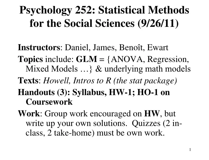
Psychology 252: Statistical Methods for the Social Sciences (9/26/11). Instructors : Daniel, James, Benoît, Ewart Topics include: GLM = {ANOVA, Regression, Mixed Models …} & underlying math models Texts : Howell, Intros to R (the stat package)

E N D
Psychology 252: Statistical Methods for the Social Sciences (9/26/11) Instructors: Daniel, James, Benoît, Ewart Topics include: GLM = {ANOVA, Regression, Mixed Models …} & underlying math models Texts: Howell, Intros to R (the stat package) Handouts (3): Syllabus, HW-1; HO-1 on Coursework Work: Group work encouraged on HW, but write up your own solutions. Quizzes (2 in-class, 2 take-home) must be own work.
Mon Sec, HW-1 and R • Our goal is to understand Statistics; access to R packages facilitates this. Expertise in Stats and R is distributed, so we’ll need to help each other. • Attention to R vs. Stats may be greater in Secs than Lectures, at least today with its ‘scrashCourse1.r’. • HW-1, due 10/05, contains review & R material, and it is ‘long’. Please start it soon. • Relevant *.r scripts in Coursework, useful for Handouts & HWs. Learning R by imitation.
Packages in R • R is a freely available language and environment for statistical computing and graphics; related to the commercial S-Plus; Google “CRAN” to get to the R homepage • Psych depts at UCLA, Virginia, etc, use it in their grad stats sequence • Stats, Poli Sci, and other Soc Sci depts at Stanford use it. • R is powerful, flexible, provides access to 3250 (in last 2 years: 2534 and 1750!) special-purpose packages, e.g., car, psy, lme4, concord, date
Lectures 1 & 2 outline • Class Project on Memory Biases: Choice of statistical analysis is influenced by our interests, the types of variables used and the design of our project.
Lectures 1 & 2 outline • Review: types of variables, key concepts, t, χ2 - appropriate terminology • Preview of GLM: ANOVA, lm(), plots, interactions; key theoretical results; contrasts; causal diagrams • R: examples
1. Class Project on memory biases • Task. Recall an instance in which you missed your plane or train, and then answer the questions on the questionnaire about how you felt, etc. • Data: Collect Pasthapp scores in R console: ‘free’, xf = c(.., …); ‘bias’, xb = c(.., …); ‘varied’, xv = c(.., …) • Collect data sheets?
2. Summary of Morewedge et al:Hypotheses • H1: correl(Pasthapp,Futurehapp) > 0. • H2: Pasthapp [free] = Pasthapp [biased] < Pasthapp [varied], • H3: Futurehapp [free] < Futurehapp [biased] = Futurehapp [varied]
Morewedge et al:Results.1 • Pasthapp [free] = 23 (S.D. = 18); Pasthapp [biased] = 20 (27); Pasthapp [varied] = 61 (31). • The group differences are significant (F(2, 59) = 16.0, p < .001), as shown by a 1-way ANOVA. Planned orthogonal contrasts are consistent with the authors’ predictions.
Morewedge et al:Results.2 • Futurehapp [free] = 31 (23); Futurehapp [biased] = 46 (26); Futurehapp [varied] = 49 (24). • The group differences are significant (F(2, 59) = 3.29, p = .044), as shown by a 1-way ANOVA. Planned orthogonal contrasts are consistent with the authors’ predictions.
Morewedge et al:Results.3 3. Correlations To get the p-values for r, I used the applet: http://faculty.vassar.edu/lowry/tabs.html
3. Testable relationships in the Class Project • Additional Hypotheses. What hypotheses might you entertain about the effects of Responsible, Changes and FTP?
Data from a previous sample • memgrp1 memgrp2 memgrp3 • 9.00 1.00 9.00 • .00 5.00 8.00 • 3.00 7.00 5.00 • 5.00 2.00 17.00 • 5.00 .00 9.00 • 5.00 3.00 15.00 • . 4.00 20.00
Possible analyses • t-tests for testing if mean for ‘memgrp1’ is the same as, or different from, mean for ‘memgrp2’; also for ‘memgrp1’ vs. ‘memgrp3’, and ‘memgrp2’ vs. ‘memgrp3’. Do an example in R console: t.test(xf, xb, paired=F, var.equal=T, na.action=na.omit) • 1-way ANOVA and the associated ‘omnibus’F test for testing if there is some difference among the 3 groups.
F-test for interaction (more interesting!): (a) Is the effect of the memory prime the same for ‘future-oriented’ people (FTP = ‘future’) as for ‘present-oriented’ people (FTP = ‘present’)? (b) Is the relation between Futurehapp and Pasthapp the same for all 3 primes? If not, we say that there is an interaction; otherwise, memory prime and Pasthapp have additive effects on Futurehapp.
Lectures 1 & 2 outline • Review: types of variables, key concepts, t, χ2 - appropriate terminology • Preview of GLM: ANOVA, lm(), plots, interactions; key theoretical results; contrasts; causal diagrams • R: examples
4. Some important ideas and distinctions • 4.1. Sample versus population
4.2. Variables • .
4.3. Relationships • The interesting questions involve a relationship between 2 (or more) variables, X and Y. For example, “Is mean(Pasthapp) equal for ‘memgrp1’ and ‘memgrp2’?” concerns a difference:“Is µ1 = µ2?”. • However, this question can be restated as, “Is there a relationship between ‘memory group’ (X) and Pasthapp (Y).” So t- and F-tests for differences can be redone using correlation and regression techniques (which we use to test for relationships).
4.3.1. A common question at the intersection of ‘difference’ & ‘relationship’ De: Ben Bolker <bbolker@gmail.com> Para: r-sig-mixed-models@r-project.org Enviado: sábado 24 de septiembre de 2011 23:02 Asunto: Re: [R-sig-ME] Factor collapsing method Iker Vaquero Alba <karraspito@...> writes: … I get a significant effect in a factor with 7 levels … but I can't know which of the levels are the most important ones in determining that effect. I have an idea from the p-values of the "summary" table, and I can also plot the data to see the direction of the effect. However, I have read in a paper that there is a method to collapse factor levels to obtain information about which factor levels differ from one another, that is used when an explanatory variable has a significant effect in the minimal model and ontains more than two factor levels. I have looked for it in the Crawley book and in the web, but I actually cannot find anything ... Discuss!
4.4. Causal Models • If X and Y are 2 variables in a data set, it is possible that • (a) X causes Y, X → Y; • (b) Y causes X, Y → X; • (c) both (a) and (b), X ↔ Y; • (d) neither (a) nor (b), X Y.
4.4.1. Mediators • Consider the SES of our parents (PSES), our own SES, and our level of education (Educ); with Educ as a mediator variable: • PSES → Educ → SES
4.4.2. Moderators • Consider PSES, our own SES, and the Type (e.g., MDC vs. LDC) of society. Suppose • cor(PSES, SES) > 0 in Type A societies, • cor(PSES, SES) = 0 in Type B societies. • i.e., PSES is uncorrelated with SES in Type B, but not Type A, societies. • Here, Type is a moderator variable; it moderates the effect of PSES on SES. Also, there is an interaction between PSES and Type in their effects on SES.
SES PSES Type Diagrams for Moderation • .
4.5. Between- and Within-subjects research designs • ‘Memory group’ is a between-subjects factor in the class project. • In contrast, we could have used a within-subjects design in which each subject is exposed to all 3 levels of the factor. Then, each level of the factor would be associated with the same group of subjects. We could compare the effects of the different primes within each participant.
Pros and Cons? Would you use a within-subject design to study ‘memory group’ effects? Why not? • The appropriate statistical analysis is different for between-subjects designs and within-subjects designs. Designs with both between-subjects and within-subjects factors are called mixed designs.
Lecture 2 outline • Review meaning of the interaction between X1 and X2 in their effects on Y. • Review of statistics involved in analysis of Memory Bias data • Definition of distribution parameters; basic theorems • Monte Carlo methods: CLT states that the distrn of is approximately Normal. For a given non-Normal popn distrn, how good is this approx? • Preview: Use ‘fieldsimul1.csv’ to preview GLM: ANOVA, lm(), plots, interactions; key theoretical results; contrasts
4.6. Measuring the interaction between 2 factors • Consider two possible ways (models) in which ‘memory group’ and Pasthapp can jointly affect Futurehapp • Additive model: differences in Futurehapp among the memory groups are approximately the same at all levels of Pasthapp. • ‘memory group’ and Pasthapp do not interact; they have additive effects on Futurehapp, and the curves are parallel. This is the critical visual (but informal) test for the absence of an interaction.
Interactive model: the differences in Futurehapp amongthe memory groups depend on the level of Pasthapp. • ‘memory group’ and Pasthapp do interact in their effects on Futurehapp. The curves are notparallel – this is the critical visual (but informal) test for the presence of an interaction. • A formal statistical test would test for the presence of an interaction (or the absence of additivity, or the non-parallelism of the curves) by means of an F-test.
Statistics from ‘Mem Bias’ project • Freq distrn, Relative freq distrn, Probability Density Function (pdf) • Boxplot: mean & variability in ‘phapp’ at each level of ‘memgrp’ • T-test: difference between 2 means • 1-way ANOVA, using lm(), the workhorse GLM function in R
T-tests • Sample of a random variable, X: x1, x2, …, xn; from which we calculate the sample mean, , st. dev., s, and variance, s2. • Z-scores (or standard scores), defined as zi = (xi – )/s. The mean of all z-scores is 0, and the s.d. is 1. ‘Large’ values of z are in the ranges ‘±2 or more extreme.’ • Linear transformations: Y = a + bX. Then, • Mean: µY = a + b µX • S.d.: σY = bσX. Variance: σY2= b2σX2
If X has a (parent) distrn, N(μ, σ2), i.e., Normal with mean, μ, and s.d., σ, then we can convert the sample mean, to a z-score or a t-score • .
T versus Z • E(Z) = 0; E(tk) = 0 (k is the df of t). • Var(Z) = 1
T-test for 2 independent samples • The null is H0: μ1 = μ2. • The alternative is H1: μ1 ≠ μ2 (2-tailed test) • The test statistic, t, is defined as follows: • The numerator of the t-ratio is the difference between the 2 sample means • The denominator is the estimate of the standard dev (also called ‘standard error’) of the difference between the 2 means • The degrees of freedom (df) of t is n1+n2-2.
T-test in R • rs1 = t.test(vf, vb, paired=F, var.equal=T, na.action=na.omit) print(rs1) • If the 2 samples were paired (and, therefore, not independent), we would use “paired=T”. • There is a test of ‘homogeneity of variance’, i.e., whether “var.equal=T”
rs1 = t.test(phapp[memgrp=='free'], phapp[memgrp=='bias'], paired=F, var.equal=T, na.action=na.omit) t = 0.914, df = 11, p-value = 0.3803 alternative hypothesis: true difference in means is not equal to 0 95 percent confidence interval: -1.911046 4.625331 sample estimates: mean of x mean of y 4.500000 3.142857
F-test for homogeneity of variance • H0 : σ12 = σ22. • H1 : σ12 ≠ σ22. • Let s12 and s22 be the variances of the 2 samples. Then the F-ratio for testing H0 is • F = max{s12, s22}/min{s12, s22}, and ‘large’ values of F (e.g., F > 4) suggest that the null should be rejected. • Because of the way F is defined, a 1-tailed test is appropriate.
F-test in R • rs1a = var.test(vf, vb, na.action=na.omit) • print(rs1a) F test to compare 2 variances F = 1.5, num df = 5, denom df = 6, p-value = 0.63 95 percent confidence interval: 0.25 10.4. This CI contains 1; therefore, we cannot reject H0.
GLM with lm() • 1-way ANOVA rs2 = lm(phapp ~ memgrp, na.action=na.omit, d0) print(summary(rs2)) • GLM with 1 categorical predictor (‘memgrp’) and 1 quantitative predictor (‘phapp’); DV is ‘future happ’, ‘fhapp’ rs3 = lm(fhapp ~ phapp + memgrp, na.action=na.omit, d0) print(summary(rs3)) #additive model rs3a = lm(fhapp ~ phapp * memgrp, na.action=na.omit, d0) print(summary(rs3a)) #interactive model
lm(formula = Futurehapp ~ Pasthapp + memtype, data = dat0, na.action = na.omit) Coefficients: Estimate Std. Error t value Pr(>|t|) (Intercept) 2.5851 1.1350 2.278 0.0280 * Pasthapp 0.3372 0.1406 2.399 0.0211 * memtypebias 0.3488 1.3500 0.258 0.7974 memtypevaried 0.1541 1.3497 0.114 0.9096 --- Residual standard error: 3.592 on 41 degrees of freedom (1 observation deleted due to missingness) Multiple R-squared: 0.1462, Adjusted R-squared: 0.08373 F-statistic: 2.34 on 3 and 41 DF, p-value: 0.08742
lm(formula = Futurehapp ~ Pasthapp * memtype, data = dat0, na.action = na.omit) Coefficients: Estimate Std. Error t value Pr(>|t|) (Intercept) 2.87262 1.04607 2.746 0.00908 ** Pasthapp 0.28684 0.17455 1.643 0.10836 memtype1 0.33030 1.31053 0.252 0.80234 memtype2 -0.33671 0.72234 -0.466 0.64371 Pasthapp:memtype1 -0.04898 0.24611 -0.199 0.84328 Pasthapp:memtype2 0.05816 0.10137 0.574 0.56947 --- Residual standard error: 3.663 on 39 degrees of freedom (1 observation deleted due to missingness) Multiple R-squared: 0.1553, Adjusted R-squared: 0.04705 F-statistic: 1.435 on 5 and 39 DF, p-value: 0.2336
Lecture 3 outline • Review of sample stats, mean, var, s.d., z-scores; and popn parameters: mean, µ, and s.d., , of a popn distrn; var( ) = 2/n • Monte Carlo methods: CLT states that the distrn of is approximately Normal. For a given non-Normal popn distrn, how good is this approx? • Preview: Use ‘fieldsimul1.csv’ to preview Chi-square tests, General Linear Model, lm(), plots, interactions; key theoretical results; contrasts
Definition of mean, var, s.d. • Popn distrn (discrete) with possible values, x1, x2, …, and associated probs, p1, p2, …, yields mean & variance: d0 = c(0:6) #x1=0, x2=1, …, x7=6 p0 = c(.1,.25,.45,.09,.07,.03,.01) #p1=.1, … mu0 = sum(d0*p0)/sum(p0) #Mean or Expected Value of X var0 = sum(p0*(d0 - mu0)^2)/sum(p0) #variance sd0 = var0^.5 #s.d. skw0 = sum(p0*(d0 - mu0)^3)/sum(p0) #skewness print(c(mean=mu0, sd = sd0, skew = skw0))
The sum, T, of n independent observations of X (HO-1, pp 12-15) • T =
The difference, D, between two independent variables • Recall the useful results on linear transformations,Y = a + bX. • Mean: µY = a + b µX • S.d.: σY = bσX. Variance: σY2= b2σX2
The Central Limit Theorem (CLT) • Under certain mild conditions on the population distrn of X, the distribution of the sample mean, tends to the Normal distrn. If we convert the sample mean into a z-score, Z, then • Z ~ N(0, 1), i.e., Z is approximately a standard Normal random variable. • If we do not know σ, then we convert the sample mean into a t score.
Sampling Distributions • Draw small (e.g., n = 9) sample from d0, compute t to test H0: µ = 1.9, say. • Convert tk to a z-score by dividing tk by its s.d., which equals . • Look at the distrn of 2000 z scores, in particular, at the mean & skewness. • Any insights?