Download
1 / 52
530 likes | 750 Views
LECTURE 9. Neural coding (2). Introduction − Topographic Maps in Cortex − Synesthesia − Firing rates and tuning curves II. The nature of neural code − Rate coding or temporal coding? ( Barn owl auditory system , place cells, and grid cells)

E N D
LECTURE 9 Neural coding (2)
Introduction • − Topographic Maps in Cortex • − Synesthesia • −Firing rates and tuning curves • II. The nature of neural code • − Rate coding or temporal coding? • (Barn owl auditory system, place cells, • and grid cells) • − Population code • • Populationcorrelation code: • (Synchrony and oscillations) • • Populationcode with statistically • independent neurons
Rate coding: • Information is encoded in the firing rate • • Temporal coding: • Precise spike timing is a significant element in neural encoding • • The debate between rate and temporal coding dominates • discussions about the nature of the neural code.
The decoding cue: the time difference between a sound reaches the two ears (the order of 0.1ms). Coincidence detector: the neuron will only be active when the inputs from two ears are received simultaneously. Accuracy 1 degree Temporal precision <5us
Remarkably enough, such a coincidence detector circuit was found four decades later by Carr and Konishi (1990) in the nucleus laminaris of the barn owl. It gives, however, no indication of how the precision of a few microseconds is finally achieved. Temporal precision is less than 5μs even though the membrane time constant and synaptic time constant are in the range of 100−1000 microseconds. How is it reached within this circuit? Interaural intensity differences (for high frequency sounds (wavelength smaller than the head) Interaural phase differences(for low frequency sounds) Delay tuning in barn owl auditory system
Place cells in rat hippocampal pyramidal cells 1 mV 200 ms Two types of theta: I and II (Skaggs et al. 1996) Examples of raw and filtered EEG. Filter bandpass: 1-100 Hz (A); 6-10Hz (B)
Place fields of place cells • Finding place cells by O’Keefe and Dostrovsky (1971) • Finding theta phase precession by O’Keefe and Recce (1993)
Theta phase precession in hippocampalpyramidal cells 0o/360o phase 270o phase (Huxter, Burgess, and O’Keefe 2003)
Theta phase precession in a place cell (Huxter, Burgess, and O’Keefe 2003)
Theta phase precessionin a place cell • Theta rhythm 7-12 Hz. • The spikes of the place cell gradually and monotonically advances to earlier phase relative to hippocampal theta rhythm as the rat traverses along the cell’s place field (Mehta, Lee and Wilson 2002)
Place cell coding in hippocampal pyramidal cells - Hippocampal place cells code the spatial position of the animal both by their firing rate and the precise timing of their firings. - A variety of different models have been developed to account for mechanisms underlying both unimodal firing profile and theta phase precession. Argument focuses on: 1) whether phase precession emerges in hippocampus itself or is inherited from upstream brain areas (Current evidences point to the latter); 2) whether dual coding is independent or inseparable (It remains unclear now).
Evidence 1:Phase precession is preserved after stimulation-induced perturbation (Zugaro, Monconduit & Buzsáki 2005)
One class of models predict that if one or both oscillators are reset, the resuming spike-phase relationship should be strongly altered by the perturbation. Thus, a simple two-oscillator model in which at least one oscillator is within the hippocampus (as opposed to the entorhinal cortex) cannot account for the present observations
Evidence 2: Phase precession in grid cells Fyhn, M., Molden, S., Witter, M. P., Moser, E. I. & Moser, M. B. Spatial representation in the entorhinal cortex. Science 305, 1258–1264 (2004) 0.3m 1.0m 0.5m 1.0m In the superficial layers of the dorsocaudal region of the medial entorhinal cortex (dMEC)
Firing fields of 3 simultaneously recorded cells (30 min running) (Hafting et al. 2005, Nature) • Spacing: 39 – 73 cm across different cells of different rats • standard deviation of spacing within a grid: 3.2 cm averaged across cells
Population data forhippocampus-independent phase precession in entorhinal grid cells (Hafting et al. 2008, Nature)
Persistence of phase precession after hippocampal inactivation in layer II cells recorded before (c) and after (d) inactivation(Hafting et al. 2008, Nature)
In summary, -Phase precession is expressed independently of the hippocampus in spatially modulated grid cells in layer II of medial entorhinal cortex, one synapse upstream of the hippocampus. -Phase precession is apparent in nearly all principal cells in layer II but only sparsely in layer III. The precession in layer II is not blocked by inactivation of the hippocampus, suggesting that the phase advance is generated in the grid cell network -The results point to possible mechanisms for grid formation and raise the possibility that hippocampal phase precession is inherited from entorhinal cortex.
How to distinguish between rate and temporal coding in practice? When precise spike timing or high-frequency firing-rate fluctuations are found to carry information, the neural code is often identified as a temporal code. The temporal structure of a spike train or firing rate is determined both by the dynamics of the stimulus and by the nature of the neural encoding process. The interplay between stimulus and encoding dynamics makes the identification of a temporal code difficult.
An MT neuron responded to the same moving random dot stimulus with the varied motion coherence c=1 c=0.5 c= 0 Another proposal is to use the stimulus, rather than the response, to establish what makes a temporal code. In this case, a temporal code is defined as one in which information is carried by details of spike timing on a scale shorter than the fastest time characterizing variations of the stimulus. (Bair and Kock 1996)
Introduction • − Topographic Maps in Cortex • − Synesthesia • −Firing rates and tuning curves • II. The nature of neural code • − Rate coding or temporal coding? • (Barn owl auditory system, place cells, • and grid cells) • − Population code • • Populationcorrelation code: • (Synchrony and oscillations) • • Populationcode with statistically • independent neurons
How is a stimulus encoded by neural activities?(Do you remember the tuning curve?) • • The discussion to this point has focused on information carried by • single neurons, but information is typically encoded by neuronal • populations • Encoding by the most active neuron sounds reasonably if there is • no noise, but it does not work in practice because of large • fluctuations in neural activities. Basically many nervous systems • use large numbers of neurons to encode information..
Population coding When we study population coding, we must consider whether individual neurons act independently, or whether correlations between different neurons carry additional information. Synchronous firing of two or more neurons is one mechanism for conveying information in a population correlation code.
Synchrony and oscillations A theory of perception --- the temporal binding. This model assumes that neural synchrony with precision in the millisecond range is crucial for object representation, response selection, attention and sensorimotor integration It defines dynamic functional relations between neurons in distributed sensorimotor networks, i.e., neurons that respond to the same sensory object may fire in temporal synchrony (Engel, Fries and Singer 2001)
An example: bistability Bistability: Two interpretations are possible of this figure (Engel, Fries and Singer 2001)
In this case, the temporal binding model predicts that neurons should dynamically switch between assemblies and, hence, that temporal correlations should differ for the two perceptual states Four visual cortical neurons with receptive fields over these four image components: the grouping which changes from one precept to another. (Engel, Fries and Singer 2001)
Neurons 1 & 2 should synchronize if the respective contours are apart of the one background face; and for neurons 3 & 4 for the candlestick. When the image is segmented into two opposing faces, the temporal coalition switches to synchrony between 1-3 and 2- 4 respectively (Engel, Fries and Singer 2001)
Introduction • − Topographic Maps in Cortex • − Synesthesia • −Firing rates and tuning curves • II. The nature of neural code • − Rate coding or temporal coding? • (Barn owl auditory system, place cells, • and grid cells) • − Population code • • Populationcorrelation code: • (Synchrony and oscillations) • • Populationcode with statistically • independent neurons
• The biggest advantage of Populationcodeis the ability to • average out noises in individual neurons if they are • independent. • Our target is to learn how a continuously moving direction is • decoded by a population of neurons. Firstly, we show two • systems: the cercal system of cricket and M1 cortex of the • monkey.
Population coding in the cercal system of cricket by a small number of neurons Crickets have two projections sticking out their posterior end: cerci. Each cercus is covered with small innervated hairs. Thousands of these primary sensory neurons send axons to a set of interneurons that relay the sensory information to the rest of the cricket’s nervous system. No single interneuron of the cercal system responds to all wind directions, and multiple interneurons respond to any given wind direction.
An interpretation from the view of statistical inference • Neural decoding is essentially a statistical inferenceprocess, • that is, to infer the stimulus value based on the observation of • data. • Consider S represents the stimulus, b the neural response, • R the noisy data. • Two phases in neural coding: • -The encoding phase: • S b • -The decoding/inference phase: • R b • Noise is ubiquitous in neural systems. • Statistical inferential sensitivity: how robust is the inferred • result with respect to noise?
Tuning curves for the four low-velocity interneurons of the cricket cercal system plotted as a function of the wind direction. rmax≈ 40 Hz. Wind speed is constant. (Theunissen and Miller 1991) At low wind velocities, information about wind direction is encoded by just four interneurons. The tuning curve for interneuron a:
Decoding the cercal system by employing the close relationship between the representation of wind direction and a Cartesian coordinate system. This vector is known as the population vector, and the associated decoding method is called the vector method. (Dayan and Abbott 2001)
Decoding arm movement direction in M1 cortex of themonkeyby population vector method Recordings fromthe primary motor cortex of amonkeyperformingan arm reaching task
Noises always exist • If the preferred directions point uniformly in all directions and the number of neurons N is sufficiently large, the population vector: Compare it with
Comparison of population vectors with actual arm movement directions (Dayan and Abbott 2001)
The neural system reads out the moving direction by the • average of preferred stimuli of all active neurons weighted by • their activities. This sounds reasonable since more active • neurons, whose preferred stimuli are more likely close to the • true stimulus, and hence should contribute more on the final vote. • Population vector demonstrated that information can be accurately • represented by the joint activities of a population of neurons in a • noise environment.. • The idea of population coding is also found in the representation of • moving direction in other parts of cortex, and the representation of • other stimuli, such as the orientation of object and the spatial • location.
Up to now, we have considered the decoding of a direction angle. We now turn to the more general case of decoding an arbitrary continuous stimulus parameter. We need use Maximum Likelihood Inference (MLI) or Bayesian inference.
An array of N neurons with preferred stimulus values distributed uniformly across the full range of possible stimulus values An array of Gaussian tuning curves spanning stimulus values from -5 to 5
Tuning curves give the mean firing rates of the neurons across multiple trials. In any single trial, measured firing rates will vary from their mean values. To implement the MLI approach, we need to know the conditional firing-rate probability density p[r|s] that describes this variability: 1. ra= na/T:the firing rate of neuron a: T:the trial duration: 2. Homogeneous Poisson model. 3. p[ra|s]: the probability of stimulus s evoking na= raT spikes, when the average firing rate is ra = fa(s)
Do you remember Poisson distribution? The probability that any sequenceof n spikes occurs within a trial of duration Tobey the Poisson distribution:
If we assume that each neuron fires independently, the firing-rate probability for the population is the product of the individual probabilities, The assumption of independence simplifies the calculations considerably.
To apply the MLI estimation algorithm, we only need to consider the terms in P[r|s] that depend on s. It is convenient to take its logarithm and write The MLI estimated stimulus, sMLI, is the stimulus that maximizes the righthand side of above equation.
On the biological plausibility of a decoding strategy • MLI, though very accurate, is often too complicated to be • implemented in neural architecture, especially, when noises are • correlated. • Population vector, may appears to be simple to computers (just • some addition and times operations), is not guaranteed to be also • simple in the view of neural systems (e.g., how to carry out these • additions and times is not obvious). Moreover, in some noise • correlation structures, population vector can be very inefficient. • In the below we will show that template-matching can be • naturally achieved in neural systems through the idea of • continuous attractor.
Attractor Computation Attractor: a steady state of a neural ensemble memorizes a stimulus value Information retrieval: a noisy input will be attracted to a steady state of the system Discrete versus continuous attractor:
The properties of continuous attractors - Continuous attractorsallows the system to change status smoothly, following a fixed path. This property (not shared by discrete attractors) is crucial for the system to seamlessly track the smooth change of stimulus -Continuous attractor seems to be most suitable for representing continuous stimulus such as the moving direction, but may also works well for encoding discrete objects if there is a continuous underlying feature linking all these objects