Download
1 / 32
320 likes | 327 Views
LESSON 4.1. MULTIPLE LINEAR REGRESSION. Design and Data Analysis in Psychology II Salvador Chacón Moscoso Susana Sanduvete Chaves. 1. INTRODUCTION. x 1. x 2. Y. x 3. x K. 1. INTRODUCTION. Model components: More than one independent variable (X): Qualitative. Quantitative.

E N D
LESSON 4.1.MULTIPLE LINEAR REGRESSION Design and Data Analysis in Psychology II Salvador Chacón Moscoso Susana Sanduvete Chaves
1. INTRODUCTION x1 x2 Y x3 xK
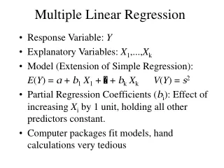
1. INTRODUCTION • Modelcomponents: • More than one independent variable (X): • Qualitative. • Quantitative. • A quantitative dependent variable (Y). • Example: • X1: educative level. • X2: economic level. • X3: personality characteristics. • X4: gender. • Y: drug dependence level.
1. INTRODUCTION • Reasons why it is interesting to increase the simple linear regression model: • Human behavior is complex (multiple regression is more realistic). • It increases statistical power (probability of rejecting null hypothesis and taking a good decision).
1. INTRODUCTION • Regression equation: Raw scores
1. INTRODUCTION • Regression equation: Deviation scores Standard scores
2. ASSUMPTIONS • Linearity. • Independence of errors: • Homoscedasticity: the variances are constant. • Normality: the punctuations are distributed in a normal way. • The predictor variables cannot correlate perfectly between them.
3. PROPERTIES The errors do not correlate with the predictor variables or the predicted scores.
4. INTERPRETATION Example 1: quantitative variables X1 0.48 Maternal stimulation 0.01 Y X2 3-year-old development level 6-year-old development level 0.62 X3 b0=20.8 Paternal stimulation
4. INTERPRETATION Example 2: quantitative and qualitative variables X1 0.157 Emotional tiredness -0.7 Y X2 Gender 0=woman 1=man Stress symptoms b0=1.987
4. INTERPRETATION The same slope, different constant = parallel lines
4. INTERPRETATION Example 3: two qualitative variables X1 -0.915 Gender 0=woman 1=man -0.096 Y X2 Work 0=public 1= private Stress symptoms b0=5.206
4. INTERPRETATION • Women, public organization: • Women, private organization: • Men, public organization: • Men, private organization:
5. COMPONENTS OF VARIATION SSTOTAL= SSEXPLAINED + SSRESIDUAL
6. GOODNESS OF FIT=COEFFICIENT OF DETERMINATION • 2 possibilities: • r12 = 0 • b) r12 ≠ 0
6. GOODNESS OF FIT=COEFFICIENT OF DETERMINATION • r12 = 0 Y a b X1 X2 X2 X1
6. GOODNESS OF FIT=COEFFICIENT OF DETERMINATION • r12 ≠ 0 Y a b c X1 X2 X2 X1 (the area c would be summed twice)
6. GOODNESS OF FIT=COEFFICIENT OF DETERMINATION Semi partial correlation coefficient square
7. MODEL VALIDATION • Null hypothesis is rejected. The variables are related. The model is valid. • Null hypothesis is accepted. The variables are not related. The model is not valid. (k = number of independent variables)
7. MODEL VALIDATION: EXAMPLE • A linear regression equation was estimated in order to study the possible relationship between the level of familiar cohesion (Y) and the variables gender (X1) and time working outside, instead at home (X2). Some of the most relevant results were the following:
7. MODEL VALIDATION: EXAMPLE • Which is the proportion of unexplained variability by the model? • Can the model be considered valid? Justify your answer (α=0.05).
7. MODEL VALIDATION: EXAMPLE • Which is the proportion of unexplained variability by the model? 2. Can the model be considered valid? Justify your answer (α=0.05). Yes, because the significance (sig.) is lower to α=0.05.
8. SIGNIFICANCE OF REGRESSION PARAMETERS • Statistic: In SPSS it is called standard error (error típico)
8. SIGNIFICANCE OF REGRESSION PARAMETERS 3. Comparison and conclusions (for each independent variable): • Null hypothesis is rejected. The slope is statistically different to 0. As a conclusion, there is relationship between variables. It is recommended to maintain the variable as part of the model. • Null hypothesis is accepted. The slope is statistically equal to 0. As a conclusion, there is not relationship between variables. It is recommended to remove the variable from the model.
8. SIGNIFICANCE OF REGRESSION PARAMETERS: EXAMPLE We studied the relationship between the variables nationality (0: Moroccan, 1: Filipino) and gender (0:man, 1:woman) with the variable depression in a 148-participant sample. We know that F is equal to 8.889, and the values obtained in the following table:
8. SIGNIFICANCE OF REGRESSION PARAMETERS: EXAMPLE • Calculate R2. • Calculate the regression equation in raw scores. • Would you remove any variable from the model? Justify your answer (α=0.05).
8. SIGNIFICANCE OF REGRESSION PARAMETERS: EXAMPLE • Calculate R2.
8. SIGNIFICANCE OF REGRESSION PARAMETERS: EXAMPLE 2. Calculate the regression equation in raw scores.
8. SIGNIFICANCE OF REGRESSION PARAMETERS: EXAMPLE 3. Would you remove any variable from the model? Justify your answer (α=0.05). No, because the t of the three parameters present a significance (sig.) lower than α=0.05