Download
1 / 46
510 likes | 711 Views
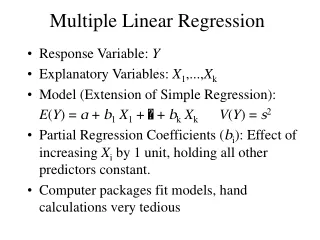
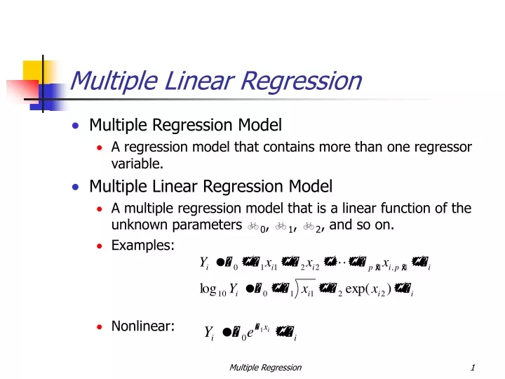
Multiple Linear Regression. Multiple Regression Model A regression model that contains more than one regressor variable. Multiple Linear Regression Model A multiple regression model that is a linear function of the unknown parameters b 0 , b 1 , b 2 , and so on. Examples: Nonlinear:.

E N D
Multiple Linear Regression • Multiple Regression Model • A regression model that contains more than one regressor variable. • Multiple Linear Regression Model • A multiple regression model that is a linear function of the unknown parameters b0, b1, b2, and so on. • Examples: • Nonlinear: Multiple Regression
Intercept: b0 Partial regression coefficients: b1, b2 Multiple Regression
Interaction: b12 can be viewed and analyzed as a new parameter b3 (Replace x12 by a new variable x3) Multiple Regression
Interaction: b11 can be viewed and analyzed as a new parameter b3 (Replace x2 by a new variable x3) Multiple Regression
Topics 1. Least Squares Estimation of the Parameters 2. Matrix Approach to Multiple Linear Regression 3. The Covariance Matrix 4. Hypothesis Tests 5. Confidence Intervals 6. Predictions 7. Model Adequacy 8. Polynomial Regression Models 9. Indicator Variables 10. Selection of Variables in Multiple Regression 11. Multicollinearity Multiple Regression
A Multiple Regression Analysis • A multiple regression analysis involves estimation, testing, and diagnostic procedures designed to fit the multiple regression model to a set of data. The Method of Least Squares The prediction equation is the line that minimizes SSE, the sum of squares of the deviations of the observed values y from the predicted values Multiple Regression
Least Squares Estimation The least square function is The estimates of b0, b1, …, bk must satisfy and Multiple Regression
1 1 . . . 1 y = X = Matrix Approach (I) Multiple Regression
Since Therefore and Matrix Approach (II) Multiple Regression
Computer Output for the Example Multiple Regression
Estimation of s2 Covariance matrix Multiple Regression
The Analysis of Variance for Multiple Regression The analysis of variance divides the total variation in the response variable y, into two portions: - SSR (sum of squares for regression) measures the amount of variation explained by using the regression equation. - SSE (sum of squares for error) measures the residual variation in the data that is not explained by the independent variables. • The values must satisfy the equation Total SS = SR + SSE. • There are (n - 1)degrees of freedom. • There are k regression degrees of freedom. • There are (n – p) degrees of freedom for error. • MS = SS /df Multiple Regression
The example ANOVA table: • The conditional or sequential sums of squares each account for one of the k = 4 regression degrees of freedom. Testing the Usefulness of the Regression Model In multiple regression, thereis more than one partial slope—the partial regression coefficients. The t and F tests are no longer equivalent. Multiple Regression
The Analysis of Variance F Test Is the regression equation that uses the information provided by the predictor variables x1, x2, …, xk substantially better than the simple predictor that does not rely on any of the x-values? - This question is answered using an overall F test with the hypotheses At least one of b 1, b 2, …, b k is not 0. - The test statistic is found in the ANOVA table as F = MSR / MSE. • The Coefficient of Determination, R2 - The regression printout provides a statistical measure of the strength of the model in the coefficient of determination. - The coefficient of determination is sometimes called multiple R2 Multiple Regression
- The F statistic is related to R2 by the formula so that when R2 is large, F is large, and vice versa. • Interpreting the Results of a Significant Regression Testing the Significance of a Partial Regression Coefficients - The individual t test in the first section of the regression printout are designed to test the hypotheses: for each of the partial regression coefficients, given that the other predictor variables are already in the model. - These tests are based on the Student’s t statistic given by which has d f = (n - p) degrees if freedom. Multiple Regression
The Adjusted Value of R2 - An alternative measure of the strength of the regression model is adjusted for degrees of freedom by using mean squares rather than sums of squares: - An alternative measure if the strength of the regression model is adjusted for degrees of freedom by using mean squares rather than sums of squares: - For the real estate data in Figure 13.3, which is provided right next to “R-Sq(adj).” Multiple Regression
Tests and Confidence Interval on Individual Regression Coefficients • Example 11-5 and 11-6, pp. 510~513 • Marginal Test Vs. Significance Test Multiple Regression
Confidence Interval on the Mean Response Multiple Regression
PREDICTION OF NEW OBSERVATIONS Multiple Regression
Measures of Model Adequacy • Coefficient of Multiple Determination • Residual Analysis • Standardized Residuals • Studentized Residuals • Influential Observations • Cook Distance Measure Multiple Regression
Coefficient of Multiple Determination Multiple Regression
Studentized Residuals Multiple Regression
Influential Observations Multiple Regression
Cook’s Distance Multiple Regression
The Analysis Procedure • When you perform multiple regression analysis, use a step-by-step approach: 1. Obtain the fitted prediction model. 2. Use the analysis of variance F test and R2 to determine how well the model fits the data. 3. Check the t tests for the partial regression coefficients to see which ones are contributing significant information in the presence of the others. 4. If you choose to compare several different models, use R2(adj) to compare their effectiveness 5. Use-computer generated residual plots to check for violation of the regression assumptions. Multiple Regression
A Polynomial Regression Model • The quadratic model is an example of a second-order model because it involves a term whose components sum to 2 (in this case, x2 ). • It is also an example of a polynomial model—a model that takes the form Example 11-13, pp. 530-531 Multiple Regression
Using Quantitative and Qualitative Predictor Variables in a Regression Model • The response variable y must be quantitative. • Each independent predictor variable can be either a quantitative or a qualitative variable, whose levels represent qualities or characteristics and can only be categorized. • We can allow a combination of different variables to be in the model, and we can allow the variables to interact. • A quantitative variablex can be entered as a linear term, x, or to some higher power such as x 2 or x3 . • You could use the first-order model: Multiple Regression
We can add an interaction term and create a second-order model: • Qualitative predictor variable are entered into a regression model through dummy or indicator variables. • If each employee included in a study belongs to one of three ethnic groups—say, A, B, or C—you can enter the qualitative variable “ethnicity” into your model using two dummy variables: Multiple Regression
The model allows a different average response for each group. • b 1 measures the difference in the average responses between groups B and A, while b 2 measures the difference between groups C and A. When a qualitative variable involves k categories, (k- 1)dummy variables should be added to the regression model. Example 11-14, pp. 534~536 <different approach> Multiple Regression
Testing Sets of Regression Coefficients • Suppose the demand y may be related to five independent variables, but that the cost of measuring three of them is very high. • If it could be shown that these three contribute little or no information, they can be eliminated. • You want to test the null hypothesis H0 : b 3=b 4=b 5 = 0—that is, the independent variables x3, x4, and x5 contribute no infor-mation for the prediction of y—versus the alternative hypothesis: H1 : At least one of the parameters b 3, b 4, or b 5 differs from 0 —that is, at least one of the variables x3, x4, or x5 contributes information for the prediction of y. Multiple Regression
To explain how to test a hypothesis concerning a set of model parameters, we define two models: Model One (reduced model) Model Two (complete model) terms in additional terms model 1 in model 2 • The test of the null hypothesis versus the alternative hypothesis H1 : At least one of the parameters differs from 0 Multiple Regression
uses the test statistic where F is based on d f1= (k-r ) and d f2=n-(k+ 1). • The rejection region for the test is identical to the rejection forall of the analysis of variance F tests, namely Multiple Regression
Interpreting Residual Plots • The variance of some types of data changes as the mean changes: - Poisson data exhibit variation that increases with the mean. - Binomial data exhibit variation that increases for values of pfrom .0 to .5, and then decreases for values of p from .5 to 1.0. • Residual plots for these types of data have a pattern similar to that shown in the next pages. Multiple Regression
Plots of residuals against Multiple Regression
If the range of the residuals increases as increases and you know that the data are measurements of Poisson variables, you can stabilize the variance of the response by running the regression analysis on • If the percentages are calculated from binomial data, you can use the arcsin transformation, • If E(y)and a single independent variable x are linearly related, and you fit a straight line to the data, then the observed y values should vary in a random manner about and a plot of the residuals against x will appear as shown in the next page. • If you had incorrectly used a linear model to fit the data, the residual plot would show that the unexplained variation exhibits a curved pattern, which suggests that there is a quadratic effect that has not been included in the model. Multiple Regression
Figure 13.17 Residual plot when the model provides a goodapproximation to reality Multiple Regression
Stepwise Regression Analysis • Try to list all the variables that might affect a college freshman’s GPA: - Grades in high school courses, high school GPA, SAT score, ACT score - Major, number of units carried, number of courses taken - Work schedule, marital status, commute or live on campus • A stepwise regression analysis fits a variety of models to the data, adding and deleting variables as their significance in the presence of the other variables is either significant or nonsignificant, respectively. • Once the program has performed a sufficient number of iterations and no more variables are significant when added to the model, and none of the variables are nonsignificant when removed, the procedure stops. • These programs always fit first-order models and are not helpful in detecting curvature or interaction in the data. Multiple Regression
Selection of Variables in Multiple Regression • All Possible Regressions • R2p or adj R2p • MSE(p) • Cp • Stepwise Regression • Start with the variable with the highest correlation with Y. • Forward Selection • Backward Selection pp. 539~549 Multiple Regression
Misinterpreting a Regression Analysis • A second-order model in the variables might provide a very good fit to the data when a first-order model appears to be completely useless in describing the response variable y. • Causality Be careful not to deduce a causal relationship between a response y and a variable x. • Multicollinearity Neither the size of a regression coefficient nor its t-value indicates the importance of the variable as a contributor of information. This may be because two or more of the predictor variables are highly correlated with one another; this is called multicollinearity. Multiple Regression
Multicollinearity can have these effects on the analysis: - The estimated regression coefficients will have large standard errors, causing imprecision in confidence and prediction intervals. - Adding or deleting a predictor variable may cause significant changes in the values of the other regression coefficients. • How can you tell whether a regression analysis exhibits multicollinearity? - The value of R 2 is large, indicating a good fit, but the individual t-tests are nonsignificant. - The signs of the regression coefficients are contrary to what you would intuitively expect the contributions of those variables to be. - A matrix of correlations, generated by the computer, shows you which predictor variables are highly correlated with each other and with the response y. Multiple Regression
The last three columns of the matrix show significant correlations between all but one pair of predictor variables: Multiple Regression