Download
1 / 32
330 likes | 482 Views
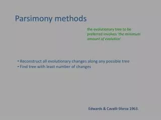
Parsimony methods. the evolutionary tree to be preferred involves ‘ the minimum amount of evolution ’. Reconstruct all evolutionary changes along any possible tree Find tree with least number of changes. Edwards & Cavalli-Sforza 1963. . A simple example.

E N D
Parsimonymethods the evolutionary tree to be preferred involves ‘the minimum amount of evolution’ • Reconstruct all evolutionary changes along any possible tree • Find tree with least number of changes Edwards & Cavalli-Sforza 1963.
A simple example Evolutionary changes: 0 1 and 1 0 Root: 0 or 1
A simple example 1 1 1 0 0 character1 Alpha Delta Gamma Beta Epsilon
A simple example 1 1 1 0 0 character1 Alpha Delta Gamma Beta Epsilon 1 0 0
A simple example 1 1 1 0 0 character1 Alpha Delta Gamma Beta Epsilon 0 1 1
A simple example 0 1 1 0 0 character2 Alpha Delta Gamma Beta Epsilon
A simple example 0 1 1 0 0 character2 Alpha Delta Gamma Beta Epsilon
A simple example 0 1 1 0 0 character2 Alpha Delta Gamma Beta Epsilon
A simple example 0 1 1 0 0 character2 Alpha Delta Gamma Beta Epsilon
A simple example 0 0 0 1 1 character3 Alpha Delta Gamma Beta Epsilon
A simple example 0 0 0 1 1 character3 Alpha Delta Gamma Beta Epsilon
A simple example 1 1 0 0 1 character4 Alpha Delta Gamma Beta Epsilon
A simple example 1 1 0 0 1 character4 Alpha Delta Gamma Beta Epsilon
A simple example 1 1 0 0 1 character 5 1 1 0 0 1 character 4 Alpha Delta Gamma Beta Epsilon
A simple example 0 1 0 0 0 character6 Alpha Delta Gamma Beta Epsilon
A simple example this first hypothesis requires a total of 9 evolutionary changes total number of changes required = 9.
A simple example colour indicates derived status ( =0, =1) Alpha Delta Gamma Beta Epsilon 6 4 5 2 5 2 4 3 characternumber 1
A simple example this alternative hypothesis requires but 8 evolutionary changes. Alpha Delta Gamma Beta Epsilon 5 5 6 4 4 2 3 1
A simple example homoplasy: the same status arises more than once on the tree Alpha Delta Gamma Beta Epsilon 5 5 6 4 4 ² 2 3 1
A simple example homoplasy: the same status arises more than once on the tree Alpha Delta Gamma Beta Epsilon 5 5 6 4 4 ² 2 3 1
Rooted and unrooted trees yet ‘another’ hypothesis requiring but 8 evolutionary changes Gamma Delta Alpha Beta Epsilon 6 5 5 4 4 ² 3 1 2
A simple example the two rooted hypotheses requiring 8 changes yield similar unrooted trees Alpha Delta Gamma Gamma Delta Beta Alpha Epsilon Beta Epsilon 6 5 5 5 5 6 4 4 4 4 ² ² 3 2 1 3 2 1
Rooted and unrooted trees Alpha Beta Gamma 5 2 3 1 5 4 4 6 Delta Epsilon
Rooted and unrooted trees unrooting trees reduces the number of alternative solutions character2 0 1 1 0 0 0 1 1 0 0 Alpha Delta Gamma Beta Epsilon Alpha Delta Gamma Beta Epsilon
Rooted and unrooted trees unrooting trees reduces the number of alternative solutions
Methods of rooting a tree Use an outgroup Use a molecular clock
Methods of rooting a tree Use an outgroup Ape3 Ape4 Ape1 root must be along this lineage Ape2 Monkey
Methods of rooting a tree only the root is equidistant to all tips Use an outgroup Use a molecular clock
Branch lengths branch lengths are computed as the sum of all character changes (each divided by # alternatives) Gamma 5 +0.5 Beta Alpha 4 +0.5 +0.5 +0.5 +0.5 2 +0.5 4 5 3 2 1 4 +0.5 2 +0.5 5 +0.5 2 +0.5 4 +0.5 6 +1 +1 +1 5 +0.5 Delta Epsilon
Branchlengths the sum of all branch lengths is called the ‘length’ of the tree Gamma Beta Alpha 1.5 0.5 1.0 1.0 2.5 1.0 1.5 Delta Epsilon
Branchlengths Gamma Beta 1.5 Alpha 0.5 1.0 1.0 2.5 1.0 1.5 Epsilon Delta
But how to… count the number of changes in large datasets reconstruct states at interior nodes search among all possible trees for the most parsimonious one handle DNA sequences (4 states) handle complex morphological characters justify the parsimony criterion evaluate statistically different trees