Download
1 / 21
210 likes | 325 Views
Comput. Genomics, Lecture 5b Character Based Methods for Reconstructing Phylogenetic Trees: Maximum Parsimony. Based on presentations by Dan Geiger, Shlomo Moran, and Ido Wexler. Modified by Benny Chor. References: Durbin et al 7.4, Gusfield 17.1-17.3, Setubal&Meidanis 6.1.

E N D
Comput. Genomics, Lecture 5bCharacter Based Methods for Reconstructing Phylogenetic Trees:Maximum Parsimony Based on presentations by Dan Geiger, Shlomo Moran, and Ido Wexler. Modified by Benny Chor. References: Durbin et al 7.4, Gusfield 17.1-17.3, Setubal&Meidanis 6.1 .
Phylogenetic Trees - Reminder • Leaves represent objects (genes, species) being compared • Internal nodes are hypothetical ancestral objects • In a rooted tree, path from root to a node corresponds to a path in evolutionary time • An unrooted tree specifies relationships among objects, but not evolutionary time
Parsimony Based Approch • Input: Character data (aligned sequences) • Goal/Output: A labeled tree (labeled internal • nodes) that “explains” the data with a minimal • number of changes across edges
AAA AAA AAA AGA AAA AAA GGA AGA AAA GGA AAG AAA AGA AAG Parsimony: An Example • Various trees that could explain the phylogeny of the following • four sequences: AAG, AAA, GGA, AGA. For example, • Parsimony prefers the second tree to the first, because it requires less substitution events(three vs. four changes).
Big and Small Parsimony • Usually the approaches to finding a maximum parsimony • tree have two separate components: • A search through the space of trees (BIG parsimony) • Given a specific tree topology, find an assignment of “ancestral labels” to internal nodes as to the minimize the total number of changes across tree edges (small parsimony)
Formally: Big Parsimony • Input: Character data (aligned sequences) • Goal/Output: A labeled tree (labeled internal • nodes) that minimizes number of changes • across edges (over all trees and internal labelings).
Formally: Small Parsimony • Input: Character data (aligned sequences) • and a tree with sequences at leaves. • Goal/Output: A labeling of internal nodes that • minimizes number of changes across edges • (over all internal labelings).
Big, Small, and Weighted Parsimony • Small parsimonyhas a linear time solution (Fitch’ algorithm). • BIG parsimony is NP hard • (easy reduction from vertex cover, VC). • Weighted small parsimony also has a linear time solution (Sankoff’s algorithm, dynamic programming).
Small Parsimony: Fitch’s Algorithm • Traverse tree “up”, from leaves to root, finding sets of possible ancestral states (labels) for each internal node. • Traverse tree “down”, from root to leaves, determining ancestral states (labels) for internal nodes. • Key observation: Different sites are independent. Can solve one site at a time.
Fitch’s Algorithm – Step 1 • Do a post-order (from leaves to root) traversal of tree • Find out possible statesRiof internal node i with children j and k
Fitch’s Algorithm – Step 1 • # of changes = # union operations T T AGT CT GT C G T T A T
Fitch’s Algorithm – Step 2 • Do a pre-order (from root to leaves) traversal of tree • Select state rj of internal node j with parent i
T T T T T T T T T T T T AGT AGT AGT AGT AGT AGT CT CT CT CT CT CT GT GT GT GT GT GT C C C C C C G G G G G G T T T T T T T T T T T T A A A A A A T T T T T T Fitch’s Algorithm – Step 2
Weighted Version • Instead of assuming all state changes are unit cost • ( equally likely), use different costs S(a,b)for • different changes • 1st step of algorithm is to propagate costs up through tree
Weighted Version of Fitch’s Algorithm • Want to determine min. cost Ri(a) • of assigning character a to node i • for leaves:
Weighted Version of Fitch’s Algorithm • want to determine min. cost Ri(a) • of assigning character a to node i • for internal nodes: a i j k b
Weighted Version of Fitch’s Algorithm – Step 2 • do a pre-order (from root to leaves) traversal of tree • select minimal cost character for root • For each internal node j, select character that produced minimal cost at parent i
Big Parsimony: Exploring the Space of Trees • We’ve considered small parsimony: How to find the minimum number of changes for a given tree topology • To solve big parsimony, need some search procedure for exploring the space of tree topologies • There are unrooted trees on n leaves
Exploring the Space of Trees taxa (n) # trees 4 15 5 105 6 945 8 135,135 10 30,405,375
Does This Implies Big MP is Hard? taxa (n) # trees 4 15 5 105 6 945 8 135,135 10 30,405,375 Not necessarily: There could be some smarter way to zoom directly to best topology. But: We will show hardness of Big MP by a (simple) reduction from vertex cover (VC).
Big MP is NP Hard ! First, define VC and VC for triangle free graphs. Then… • You will show a poly time reduction from VC to VC for triangle free graphs as part of home assignment(easy). • In class,I will show a poly time reduction from • VC for triangle free graphs to Big MP • (old style, white board proof). • This establishes NP hardness of Big MP.