Download
1 / 1
10 likes | 171 Views
VAR(U). VAR(Y). VAR(X). A. B. C. VAR(Z). The Theory and Practice of Instrumental Variable Estimation Dan Hammer ’07 Swarthmore College, Department of Mathematics & Statistics. Empirical Examples in Economics

E N D
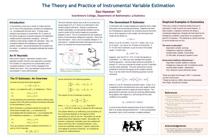
VAR(U) VAR(Y) VAR(X) A B C VAR(Z) The Theory and Practice of Instrumental Variable Estimation Dan Hammer ’07 Swarthmore College, Department of Mathematics & Statistics Empirical Examples in Economics There are a variety of empirical studies that use IV estimation in order to parse out causal impacts. In these studies, a regressor central to the study is considered endogenous. Analysts will instrument for the endogenous variables, using theory as a jumping-off point for IV selection. The following is a (brief) overview of recent studies that use IVs: The return to education*: Dependent variable: earnings Endogenous regressor: education Unobservable variable: innate ability IV: birth date, according to quarter of year Government healthcare effectiveness**: Dependent variable: epidemic outbreak Endogenous regressor: dist. to healthcare center Unobservable variable: “cleanliness” IV(s): distance to post office/train station *Study by Angrist and Krueger (1991), in Quarterly Journal of Economics **Study by Hammer (2006), Advanced Econometrics Term Paper, Swarthmore College The Generalized IV Estimator IV estimation with a single endogenous regressor and a single instrument can be naturally generalized. Suppose that there are K endogenous regressors (for simplicity assume that there are no other regressors in the model); then the benchmark model can be written as where X is an N x K matrix; y is an N x 1 matrix; and ε is an N x K matrix. Let Z be an N x R matrix of instruments. If K = R, then the IV estimator is just as it was in the simple model. In matrix form: Suppose, now, that R ≠ K. If R < K, then the equation is unidentified – i.e., there are more variables than sample moment equations – and the model cannot be estimated. If, instead, R > K we can evaluate the model, but the IV estimator must be further specified. The extra instruments must be combined to minimize the square of the sample moments. Thus, it can be shown that the following quadratic must be minimized: where Wn is an R x R positive symmetric matrix. In fact, Wn is a weighting matrix that determines how much weight to place on each sample moment to satisfy the best fit criterion. The generalized IV estimator can then be solved by differentiating the quadratic with respect to β, and solving the first order conditions, thus yielding: It can be shown that the expected value of the IV estimator – both in its simple and generalized form – is the true population parameter; that is, the IV estimator is indeed unbiased. Introduction In econometrics, there are a variety of models wherein one or more of the explanatory variables are endogenous (i.e., correlated with the error term). In these cases, analysts must employ an econometric “fix” to parse out the strictly exogenous covariation between the dependent variable and the explanatory variable(s). One such method is instrumental variable (IV) estimation. Here, the covariation between the endogenous regressor and another variable – that would otherwise be excluded from the model – is utilized to consistently estimate the model’s parameters. An IV Heuristic Each circle in Figure 1 represents variation in the specified variable; common area represents covariation. The variable U is assumed to be unobservable; that is, covariation between Y and U will be relegated to the model’s error term. Thus, any estimator using common area between Y and U will be biased. The OLS estimator utilizes area (A+B+C) to assess the causal impact of X on Y; there is no information in the model to specify otherwise. Instead, to estimate the model’s parameters, an instrumental variable Z can be used to cordon off the strictly exogenous covariation between X and Y. The IV is projected onto the exogenous portion of the otherwise endogenous regressor. Given this new information – that is, the tri-covariation between Y, X, and (now) Z – standard estimation techniques will use only area C to evaluate the structural parameters. Figure 1: The IV is projected onto the endogenous regressor, isolating exogenous covariation. The IV Estimator: An Overview Consider the linear benchmark equation: where x1i is exogenous; and x2iis endogenous. That is, so that estimating the benchmark model by ordinary least squares (OLS) will yield inconsistent and biased estimates for the parameters β1andβ2. More information is needed to identify the model: An instrumental variable (say, z2i) is assumed to be uncorrelated with the model’s error εi, but correlated with the endogenous regressor x2i. In symbolic notation: Thus, by using the moment conditions derived from (1) and (4), the IV estimator can be solved from the following equations The solution for the IV estimator is given by: where and . Note that if , then the IV estimator is exactly the OLS estimator. The relative efficiency (or inefficiency) and consistency of the IV estimator depends on the degree to which assumptions (3) and (4) are met. Assumption (3) can be tested using linear regression models. Assumption (4), however, is generally untestable: given the unobserved nature of the error term, correlation between εiand zi cannot be analytically assessed. Instead, researchers must appeal to economic reasoning – an unsatisfying recourse for mathematicians. References Bowden, R. & Turkington, D. (1984). Instrumental Variables. New York: Cambridge University Press. Davidson R. & MacKinnon J. (1993). Estimation and Inference in Econometrics. New York: Oxford University Press. Greene, W. (1993). Econometric Analysis (2nd ed.). New York: Macmillan Publishing Company. Koutsoyiannis, A. (1977). Theory of Econometrics (2nd ed.). London: Macmillan Publishing Company. Spanos, A. (1986). Statistical Foundations of Econometric Modelling. New York: Cambridge University Press. Verbeek, M. (2005). Modern Econometrics (2nd ed.). West Sussex, England: John Wiley & Sons, Ltd. Acknowledgements I want to thank Professor Jefferson for his IV heuristic – and the rest of his help, actually. Additionally, I want to thank Professor Stromquist for his help working through the geometry of least squares estimation.