Download
1 / 47
470 likes | 684 Views
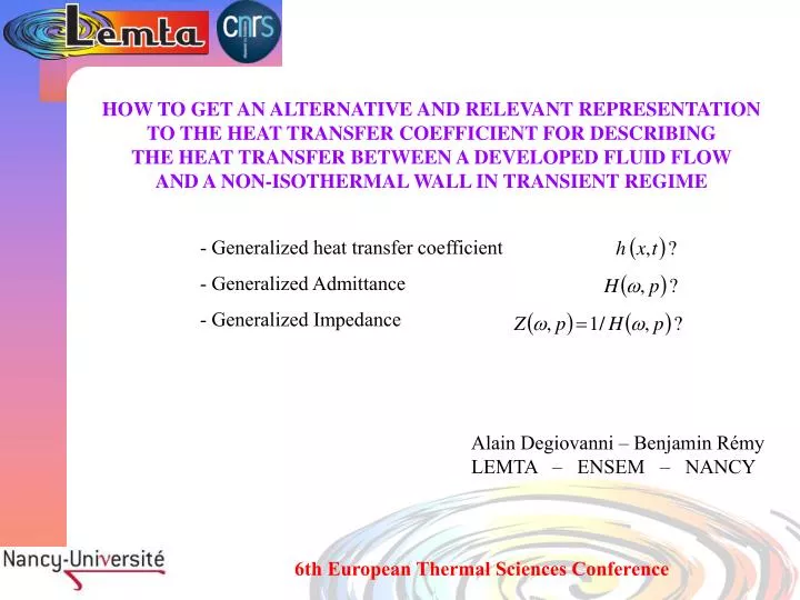
HOW TO GET AN ALTERNATIVE AND RELEVANT REPRESENTATION TO THE HEAT TRANSFER COEFFICIENT FOR DESCRIBING THE HEAT TRANSFER BETWEEN A DEVELOPED FLUID FLOW AND A NON-ISOTHERMAL WALL IN TRANSIENT REGIME. Generalized heat transfer coefficient Generalized Admittance Generalized Impedance.

E N D
HOW TO GET AN ALTERNATIVE AND RELEVANT REPRESENTATION TO THE HEAT TRANSFER COEFFICIENT FOR DESCRIBING THE HEAT TRANSFER BETWEEN A DEVELOPED FLUID FLOW AND A NON-ISOTHERMAL WALL IN TRANSIENT REGIME • Generalized heat transfer coefficient • Generalized Admittance • Generalized Impedance Alain Degiovanni – Benjamin Rémy LEMTA – ENSEM – NANCY 6th European Thermal Sciences Conference
OUTLINE I) GENERAL PROBLEM II) FLAT PLANE IN STEADY-STATE REGIME III) FLAT PLANE IN TRANSIENT REGIME IV) PLUG FLOW IN STEADY-STATE REGIME V) GRAETZ PROBLEM VI) AXIAL DIFFUSION VII) PLUG FLOW IN TRANSIENT REGIME VIII) CHILTON-COBURN CORRELATION IX) APPLICATION: THICK WALL
INTRODUCTION at solid-fluid interface in steady-state regime h heat transfer coefficient (1/h is a resistance) and heat flux density and surface temperature reference temperature in a flux tube in steady-state regime In transient regime
A heat flux tube in transient regime (thermal equilibrium) After a Laplace transform in t : 3 Impedances
Assuming a semi-infinite medium : with We can always write: depends on but is independent of since
at I – GENERAL PROBLEM independant of x and t in in or any kind of condition in Figure 1
I –SOLUTION After a double transform: The problem becomes: General solution is given by: If the boundary condition in y=e is fixed:
General form: thus : and not : in the case where: and independant of the boundary condition in y = 0
PROBLEM SOLUTION II – FLAT PLANE IN STEADY-STATE REGIME With uniform velocity field and negligeable conduction is x After a Laplace transform in x : and consequently Independant of the boundary conditions Figure 2
II – CLASSICAL APPROACH Let calculate h(x) from its definition : - Uniform imposed temperature: - Uniform imposed heat flux: h(x) depends on the Boundary Conditions
In particular, let calculate h(x) for an imposed localized heat flux between a < x < b:
j = j 0 = T T 0 ( ( ) ( ) ) j = j g - - g - x a x b 0 II – RESULTS h(x) for The extension to a non-uniform velocity field U(y) can be carried out without major difficulties expect the complexity of the solution
PROBLEM SOLUTION III – FLAT PLANE IN TRANSIENT REGIME After a double Laplace transform in x and t (p and s) : independant of the boundary conditions
IV – PLUG FLOW IN STEADY-STATE REGIME PROBLEM: SOLUTION: After a Laplace transform in x that is
Calculation of the impedance: • Usually, heat transfer is evaluated using the average fluid bulk temperature (bulk temperature) as reference: thus : with this yields: with Independant of the boundary conditions
( ) h x j and consequently - Calculation of let by definition and that is: The limit for established regime is given by:
( ) h x T - Calculation of let: by definition and that is: and consequently with that can be written We numerically obtain the limit of
( ) j = j = j = j j = j g - T T x b 0 0 0 0 RESULTS : Nu Nu X* X* Figure 7 : Plug flow Nu(x*) with Figure 6 : Plug flow Nu(x*)with (b* = 0.1)
V – GRAETZ PROBLEM The proposed method allows us to solve the GRAETZ problem for any types of imposed boundary conditions at the tube wall, through only one calculation -PROBLEM: with
SOLUTION : • After a Laplace transform, with The solution is: with and by definition: with this yields:
and (the same for plug flow) heat transfer coefficients for After calculation of we obtain: and and consequently:
Notice: Laplace inversions are particularly difficult to perform (the solution depends on a complex variable) The solution consists in using the Cauchy's residue theorem. Solutions appears as exponential series. After calculation, we obtain for and with
( ( ) ) h h x x : : j T Calculation of uniform heat flux Calculation of uniform imposed temperature with
j = j 0 = T T 0 Nu RESULTS : Laminar flow Nu(x) X* Laminar flow (parabolic velocity profile)
VI –AXIAL DIFFUSION Axial diffusion can easily be taken into account; as for instance in the case of the plug flow: After a Laplace transform in x The solution is:
VII – PLUG FLOW IN TRANSIENT REGIME Let consider the plug flow problem: After a double Laplace transform in x and t:
and consequently: For instance, let calculate h(x,t) for a uniform flux in space and in time: and consequently
RESULTS : Figure 10 Figure 11 a = 0.07, b = 0.01, c = 0.07
VIII – CHILTON – COLBURN CORRELATION Another interest of the method: Calculation of the impedance from a given correlation h(x,t) obtained in the case of a particular boundary condition, using an inverse method. This correlation being obtained either from a calculation/computation or by experiment Application : Chilton – Colburn correlation * A correlation for a given boundary condition is chosen, * The transfer function is estimated from it, * The correlations for any types of boundary conditions are calculated from the estimated transfer function
- General relations between h(x) and Z(p) for - General relations between h(x) and Z(p) for
VIII – LAMINAR REGIME - In the case or that is: This impedance does not depend on the boundary conditions
- Let calculate from this, the correlation for to compare with solution found in literature
- And the correlation for a heaviside heat flux that is Figure 4 consequently that is with
This yields to a correction term to compare with literature reference C x correction for a heaviside heat flux (b = 2)
VIII – IN TURBULENT REGIME Let use the imposed temperature correlation for the impedance calculation: Applying the same technique, we obtain the impedance: and consequently the correlation in the case of imposed heat flux to compare with literature result :
IX – APPLICATION The proposed approach is particularly of interest when an interaction between the fluid and the wall exists (in microfluidics for instance). In this case, the heat flux distribution at the interface is unknown and only the proposed method allow us to solve the problem. In the cases of complex geometries for which numerical computations are required, the convolution product must be used. In the general case: If the geometry is simple and the integral transforms applicable, the generalized impedance can be used; after transformation:
Flat plate submitted to a local heat flux on its lower face and in contact on its upper face with a moving fluid with a uniform velocity field (Plug Flow) PROBLEM:
SOLUTIONS: Numerical solution of the complete problem (fluid + wall) by a finite element code (Flex PDE) Analytical solution by replacing the fluid by its impedance Z(p) Numerical solution by replacing the fluid by a classical correlation h(x)
ANLYTICAL SOLUTION: After a Laplace transform in x :
RESULTS: Figure 13
Comparison convolution product-numerical methods Air v = 1m/s a = 0.5 b = 1 Wall Temperatures Wall Temperatures 16 14 Numerical Numerical . 14 Impedance Impedance 12 12 10 10 = 0.1 = 1 8 8 Temperatures Temperatures 6 6 4 4 2 2 0 0 -2 -2 0 0.5 1 1.5 2 2.5 3 3.5 4 0 0.5 1 1.5 2 2.5 3 3.5 4 x x Wall Temperatures 14 Wall Temperatures Numerical 10 Impedance Numerical 12 Impedance 8 10 8 6 = 5 = 50 Temperatures 6 Temperatures 4 4 2 2 0 0 -2 0 0.5 1 1.5 2 2.5 3 3.5 4 -2 x 0 0.5 1 1.5 2 2.5 3 3.5 4 x
Wall Temperatures for different heat transfer coefficients 12 h = constante - h = k*x 1/2 10 - h = k*(x-a) 1/2 h = impedance 8 Temperatures 6 4 2 0 0 50 100 150 200 250 300 350 400 x
Wall Temperatures for different heat transfer coefficients 20 h = constante 18 - h = k*x 1/2 - h = k*(x-a) 1/2 16 h = impedance 14 12 Temperatures 10 8 6 4 2 0 0 50 100 150 200 250 300 350 400 x
Wall temperatures for different heat transfer coefficients 18 h = constante 16 - h = k*x 1/2 - h = k*(x-a) 1/2 14 h = impedance 12 10 Temperatures 8 6 4 2 0 -2 0 50 100 150 200 250 300 350 400 x
CONCLUSION I have tried to convince you that the most adapted model to use to take into account the thermal coupling between a solid and a fluid is to introduce a generalized impedance instead of a heat transfer coefficient varying in space and time. Indeed it is intrinsic to the fluid and it does not particulary depend on the thermal boundary conditions and on the solid thermal properties. Its implementation is quite easy because we only need to introduce it as a convolution product in the wall boundary condition. Examples have been shown here for simple cases ; for more complex cases, this impedance cannot be calculated analytically as it was done in this work but it can be estimated expe- rimentally by inverse technique using infrared thermography measurements for example. Only one experiment is required to obtain the impedance of a system that can be used thereafter for simulating thermal response of this system to any other types of thermal boundary conditions.
Thankyou for your attention !!!