Download
1 / 64
640 likes | 935 Views
The Causes of Variation. Lindon Eaves and Tim York Boulder, CO March 2001. One Issue (Among Many!). Identifying genes that cause complex diseases and genes that contribute to variation in quantitative traits. Quantitative Trait Locus (QTL).

E N D
The Causes of Variation Lindon Eaves and Tim York Boulder, CO March 2001
One Issue (Among Many!) • Identifying genes that cause complex diseases and genes that contribute to variation in quantitative traits
Quantitative Trait Locus (QTL) Any gene whose contribution to variation in a quantitative trait is large enough to stand out against the background noise of other genetic and environmental factors
Quantitative Trait A continuously variable trait (in which variation may be caused by multiple genetic and/or environmental factors); any categorical trait in which differences between categories may be mapped onto variation in a continuous trait
Common diseases • Estimated life time risk c.60% • Substantial genetic component • “Non-Mendelian” inheritance • Non-genetic risk factors • Multiple interacting pathways • Most genes still not mapped
Examples • Ischaemic heart disease (30-50%, F-M) • Breast cancer (12%, F) • Colorectal cancer (5%) • Recurrent major depression (10%) • ADHD (5%) • Non-insulin dependent diabetes (5%) • Essential hypertension (10-25%)
Even for “simple” diseases:Number of alleles is large(Wright et al, 1999) • Ischaemic heart disease (LDR) >190 • Breast cancer (BRAC1) >300 • Colorectal cancer (MLN1) >140
Definitions • Locus: One of c. 30-40,000 genes • Allele: One of several variants of a specific gene • Gene: a sequence of DNA that codes for a specific function • Base pair: chemical “letter” of the genome (a gene has many 1000’s of base pairs) • Genome: all the genes considered together
Finding QTLs • Linkage • Association
Linkage Finds QTLs by correlating phenotypic similarity with genetic similarity (“IBD”) in specific parts of genome
Linkage • Doesn’t depend on “guessing gene” • Works over broad regions (good for getting in right ball-park) and whole genome (“genome scan”) • Only detects large effects (>10%) • Requires large samples (10,000’s?) • Can’t guarantee close to gene
Association • Looks for correlation between specific alleles and phenotype (trait value, disease risk)
Association • More sensitive to small effects • Need to “guess” gene/alleles (“candidate gene”) or be close enough for linkage disequilibrium with nearby loci • May get spurious association (“stratification”) – need to have genetic controls to be convinced
“Reality”:For complex disorders and quantitative traits Large number of alleles at large number of genes
Defining the Haystack • 3x10⁹ base pairs • Markers every 6-10kb for association in populations with no recent bottleneck history • 1 SNPs per 721 b.p. (Wang et al., 1998) • c.14 SNPs per 10kb = 1000s haplotypes/alleles • O (104 -105) genes
Problems • Large number of loci and alleles/haplotypes • Possible interactions between genes • Possible interactions between genes and environment • Relatively low frequencies of individual risk factors • Functional form of genotype-phenotype relations not known • Sorting out signal from noise – minimizing errors within budget • Scaling of phenotype (continuous, discontinuous) • Spurious association (stratification)
Prepare for the worst Need statistical approaches that can screen enormous numbers of loci and alleles to identify reliably those that have impact on risk to disease
System Chosen for Study • 100 loci • 20 loci affect outcome, 80 “nuisance” genes • 257 alleles/locus • Allele frequencies c.20-0.1% • Disease genes each explain 2.5% variance in risk (c. 2-fold risk increase) • 40% rarest alleles increase risk • 50% variance non-genetic
It’s a Mess! • Don’t know which genes – might have clues • Don’t know which alleles – unordered categories • >250100 locus/allele combinations • More predictor combinations than people (“curse of dimensionality”) • Reality worse
Problems • Informatics: large volume of data • Computational: large number of combinations • Statistical: large number of chance associations • Genetic-epidemiological: secondary associations
Data Mining(Steinberg and Cartel) • Attempt to discover possibly very complex structure in huge databases (large number of records and large number of variables) • Problems include classification, regression, clustering, association (market analysis) • Need tools to partially or fully automate the discovery process • Large databases support search for rare but important patterns and interactions (epistasis, GxE)
Some Approaches to DM • Logistic regression • Neural networks • “CART” (Breiman et al. 1984) • “MARS” (Friedman, 1991)
“MARS” • Multivariate • Adaptive • Regression • Splines
Key references Friedman, J.H. (1991) Multivariate Adaptive Regression Splines (with discussion), Annals of Statistics, 19: 1-141. Steinberg, D., Bernstein, B., Colla, P., Martin, K., Friedman, J.H. (1999) MARS User Guide. San Diego, CA: Salford Systems
The MARS Advantage • Allows large number of predictors (loci/alleles/environments) to be screened • Non-parametric • Continuous and discontinuous outcomes • Systematic search for detailed interactions • Testing and cross-validation • Continuous and categorical predictors • Decides best form of relationship
Example Regression Spline:Impact of Non-Retail Business on Median Boston House Prices Median House Price “Knot” Industrial Business
Fitting functions with Splines • Piece-wise linear regression. • simplest form. allow regression to bend. • “Knots” define where the function changes behavior. • Local fit vs. Global fit. actual data spline with 3 knots
One predictor example True knots at 20 and 45 (left) Best single knot at about 35 (right) Y Y 10 20 30 40 50 60 10 20 30 40 50 60 X X
10 20 30 40 50 60 10 20 30 40 50 60 10 20 30 40 50 60 10 20 30 40 50 60
Re-express variables as basis functions • Done to generalize the search for knots. Difficult to illustrate splines with > one dimension. • Core building block of MARS model • max (0, X – c); • example: BF1 = max(0, ENV – 5); BF2 = max(0, ENV – 8); 0 for ENV <= 5; 1 for 5 <= ENV <= 8; 1 + 2 for ENV > 8; • Weighted sum of basis functions used to approximate the global function. • ie y = constant + 1 * BF1 + 2 * BF2 + error;
“Adaptive” Spline • “Optimal” placement of knots • “Optimal” selection of predictors and interactions
Adaptive splines • Problem: • What is the optimal location of knots? • How many knots do you need? • Best to test all variable / knot locations, but computationally burdensome. • MARS solution: • Develop an overfit model with too many knots. • Remove all knots that contribute little to model quality. • The final model should have approximately correct knot locations.
“Optimal” Explains “salient” features of data Ignores irrelevant features Stands up to replication - Several ways to operationalize mathematically
MARS 2-step model building • Step 1.Growing phase: • begins with only a constant in the model. • serially adds basis functions to a user defined limit. tests each for improvement when added to the model. • addition of basis functions until an overly large model is found. (theoretically the true model is captured). • Step 2. Pruning phase: • delete basis function that contributes least to model fit. • refit the model and delete next term, repeat. • the most parsimonious model is selected. • GCV criterion to select optimal model (Craven 1979). • MARS option uses 10 fold cross-validation to estimate DF.
Cross-validation • Protects against over fitting data. • Develops a model on subset of data. Tests fit on remaining set. • Systematically assesses how many DF to charge each variable entered into model. • Adding a basis function will always lower MSE. • This reduction is penalized by DF charged. • Only backwards deletion step is penalized.
So Far: Does quite well for largish random samples and continuous outcomes. -What about disease (dichotomous) outcomes? -What about selected (extreme) samples?
So? • Can detect signal due to relatively large numbers of relatively rare unordered alleles of relatively small effect at relatively many loci amid the noise of still more loci and environmental effects • “MARS” may provide elements for analyzing such data in this and similar contexts (?micro- arrays, SNPs, expression arrays?) • Works with continuous data on random samples and dichotomous outcomes on selected samples