Download
1 / 31
310 likes | 329 Views
This agenda outlines the use of AFT and FSI tools for validating components of interest rate risk models, including prepayment models, stochastic rate generators, and aggregators.

E N D
Using AFT and FSI Tools to Validate Components of Interest Rate Risk Models
Agenda • Validation Tests of Prepayment Models • Models applicable to securities • Models applicable to portfolio loans • Validation Tests of Stochastic Rate Generators using FSI • Lattice • Monte Carlo
Regressor and Back-testing • Regressor is applicable to AFT prepayment models: • Securities • MBS • CMOs • MBS data at the CUSIP level require extraction routines from Bloomberg or Intex. • CMO data at the CUSIP level require license with Intex, Chasen or other cash flow model vendor. • Agency CMO data can be extracted from Bloomberg.
Regressor and Back-testing • Batch “Back-test” in the Regressor Model • Output created: • Actual CPR • AFT forecast of CPR using actual rates • Output is written to text files with number of files equal to the number of collateral types. • Example: 300 CUSIPs of 15 and 30 FNMA, FHMLC, and Whole loans might reside in six text files • All CUSIPs can be run at once in Regressor with the text files created automatically. • Text files can be opened in EXCEL and standard “goodness of fit” or other statistics applied.
Regressor and Back-testing • Once a macro is written, process takes less than an hour for the entire list of CUSIPs (We did this for 300 CUSIPs.) • Procedure can be learned in about 15 minutes via phone support, if all required extract files are available. • Regressor allows the aggregation across CUSIPs drawn from same collateral. Performance on sub-portfolios can be assessed.
Why can AFT Claim Regressor Provides a Back-test”? • AFT Prepayment models are estimated using collateral data • Securities are small samples of the collateral. • Output in Regressor at CUSIP level is based on both overlapping historical periods and projected periods, depending on the length of history and when collateral model was estimated. • Over the historical data model period this is an “in-sample” back-test. • When CPRs are projected beyond historical data period used for building models, the test is an “out-of-sample” back-test. • If the connectivity in the ALM system and AFT models has been validated, then the ALM model is not needed for back-testing AFT prepayment models.
Back testing Sample Output from Regressor One of 180 graphs created for an ALCO Partners client
Dynamic Aggregator and Back testing • Dynamic Aggregator is applicable to portfolio loans • Similar output created as in Regressor • AFT prepayment models provide the basis for modeling. Discrete prepayment factors can be scaled to improve model fit. • Historical data used to fit model and model statistics can be created as part of the estimation process. • In-sample and out-of-sample model testing can be applied with similar statistics. • If AFT-ALM model link has been validated, then the process can substitute for back test using ALM model.
Findings from Dynamic Aggregator Projects • Dynamic Aggregator has coincidentally “solved” a classic data bottleneck in many banking institutions • IT departments now regularly archive historical data relevant for testing prepayment models • They are very efficient at providing raw data. • They are inefficient at “mapping” data • Internal resources for “research and analysis” are frequently low on a priority list • External projects where only raw data is required appear not to face the same internal hurdles because they demand very few IT resources
Findings from Dynamic Aggregator Projects • A part of prepayment model validation projects applicable to portfolio mortgages is obtaining and mapping data. But this process is no longer a large cost. • Mapping costs have not been large. Key variable is number of systems • Mapping rules typically remain constant over time, so annual updates become very cost effective • Once the data has been mapped into Dynamic Aggregator, the process for testing and is very cost-effective, particularly when the process is done annually as required by banking regulations
Testing Stochastic Rate Generators • In many banks stochastic rate generators are being utilized to measure value based IRR • Base case is calibrated to market instruments • There are known nuances and problems associated with this • How does a bank “validate” a stochastic rate model?
Testing Stochastic Rate Generators • Approach I • Obtain model documentation • Build a separate model independently • Perform double-blind tests and compare inputs and outputs • Issues with Approach I • Vendors may be unwilling to provide proprietary code documentation • Building a separate model can be very expensive, including its validation • Specialized coding/math expertise required to “build” a stochastic rate generator
Testing Stochastic Rate Generators • Approach II • Obtain a qualified stochastic rate generation system • Calibrate to the same set of market instruments • Compare inputs and outputs for tested samples • FSI: A qualified stochastic rate generation system
Testing Stochastic Rate Generators • FSI is a fully specified two factor lattice & Monte-Carlo system designed as a portfolio management product with validation capabilities • Provides a basis for comfort or discomfort depending on the model results and how the model results are integrated with portfolio management decisions • Since it contains both single factor (BK) and two-factor processes, it provides a basis for understanding the sensitivity of the risk measure to the underlying process utilized • Helps improve calibration procedures and allows a look into the “black box” of stochastic rate generation capability
Testing Stochastic Rate Generators • Test Procedures • Compared stochastic output from a widely used ALM model with a stochastic generator • Compared three portfolios in two periods • MBS & CMO • Portfolio FRMs • Callable Bonds • Greeks are computed at the instrument level • Market values and market values under rate shocks can be computed • Market values changes compared over time at instrument level • Results used to refine and understand calibration process and reasonableness of risk results
Callables: MV Sensitivity 12/31 3/30 Callables: MV Sensitivity Compared Callables: MV Sensitivity Compared 8% 8% FSI1F FSI1F 6% 6% FSI2F FSI2F ALM 4% 4% ALM MV MV 2% 2% % D % D 0% 0% -2% -2% -4% -4% -6% -6% -150 -100 0 100 150 200 -150 -100 0 100 150 200 Shock (bp) Shock (bp) Market value sensitivity measures for callable bond portfolio where very similar in both time periods
Callables: FSI 2F vs. ALM Model Callables: FSI 2F vs. ALM Model 8 8 7 6 6 5 4 Duration (ALM) Convexity (ALM) 4 2 3 2 0 1 0 -2 0 1 2 3 4 5 6 7 8 -2 0 2 4 6 8 Duration (FSI 2Factor) Convexity (FSI 2Factor) Callables: Duration & Convexity Duration Convexity Red line represents parity Results indicated some non-random differences on individual securities. Further investigation revealed pattern associated with “at the money” calls. Cross checks with market values showed sensitivity to calibration mechanics
Callables: 3/31 vs. 12/31, FSI vs. ALM Model 4% 3% 2% MV (ALM) 1% D % 0% -1% -1% 0% 1% 2% 3% D % MV (FSI 2Factor) Callables: FSI 2 Factor vs. ALM Model: 12/31 to 3/31 How does Market Value Change over Time? Red line represents parity
FRMs: MV Sensitivity 12/31 3/31 FRMs: MV Sensitivity FRMs: MV Sensitivity 6% 4% 4% 2% 2% 0% 0% MV MV -2% -2% FSI1F %D %D FSI1F FSI2F -4% -4% FSI2F ALM -6% ALM -6% -8% -8% -10% -10% -12% -150 -100 0 100 150 200 -150 -100 0 100 150 200 Shock (bp) Shock (bp) Prepayment models were identical
FRMs FRMs 6 0 5 -1 4 -2 Duration (ALM) Convexity (ALM) 3 -3 2 -4 1 0 -5 0 1 2 3 4 5 6 -5 -4 -3 -2 -1 0 Duration (FSI 2Factor) Convexity (FSI 2Factor) FRMs: Duration & Convexity Duration Convexity Red line represents parity
FRMs 0% -1% MV (ALM) D -2% % -3% -3% -2% -1% 0% D % MV (FSI 2Factor) FRMs: FSI (2 Factor) vs. ALM: 12/31 to 3/31 Red line represents parity FRMs where there are good market value indicators combined with the OAS calculations lead to similar results
CMOs & MBS: MV Sensitivity 12/31 3/31
CMOs & MBS: Duration & Convexity Duration Convexity Red line represents parity Circled outliers were later identified as input errors in the ALM model
CMOs & MBS: FSI (2 Factor) vs. ALM: 12/31 to 3/31 Red line represents parity Four outliers are the same CUSIPs as in the prior graph
Yield Curve Distributions: Single Factor vs. Two Factor Stochastic Processes Single Factor Process: Yield Curve Distribution
Yield Curve Distributions: Single Factor vs. Two Factor Stochastic Processes Two Factor Process: Yield Curve Distribution
Yield Curve Distributions: Single Factor vs. Two Factor Stochastic Processes Two Factor Process: Yield Curve Distribution Single Factor Process: Yield Curve Distribution
FRMs: MV Sensitivity: Single vs. 2 Factor 12/31 3/31 FRMs: MV Sensitivity FRMs: MV Sensitivity 6% 4% 4% 2% 2% 0% 0% MV MV -2% -2% FSI1F %D %D FSI1F FSI2F -4% -4% FSI2F ALM -6% ALM -6% -8% -8% -10% -10% -12% -150 -100 0 100 150 200 -150 -100 0 100 150 200 Shock (bp) Shock (bp) Impact of process is limited in this case even though distribution of yield curves is noticeable
Observations from Test • Stochastic models will frequently produce different measures of risk at the instrument level for instruments with embedded options • We believe – but it is difficult to confirm without access to source code – that this is largely due to differences in calibration procedures as well as differences in modeling methods. • With larger portfolios that include instruments with a wide variety of option structures, the differences in results will tend to cancel each other out if the overall levels of implied volatility used in the calibrations are similar.
Observations from Test • Validation tests of stochastic models using a qualified stochastic model, such as FSI, can: • Identify modeling errors, because large differences in results invite further investigation • Enhance understanding of the “black box” of ALM model calibration procedures, when calibrations aren’t “all that close” • Provide guidance for the product characteristics that are stochastic modeling technique sensitive • Validation tests of stochastic models lead to the following warning: Beware of relying on a single stochastic model when measuring risk at the instrument level for instruments with embedded complex options
Observations from Test • Tests of stochastic models can identify modeling errors, because large differences invite further investigation • Word to the warning about using stochastic models for risk management involving individual transactions