Download
1 / 25
260 likes | 345 Views
q. f. z. R. z. x. y. r. f. . . . Length, Area,Volume. Spherical. Rectangular. Cylindrical. dl 2 = dR 2 + R 2 d f 2 + R 2 sin 2 q dz 2 dA r = (R d q ).(Rsin q d f ) dA q = dR.(Rsin q d f ) dA f = dR.Rd q dV = R 2 sin q dR.d q .d f. dl 2 = dx 2 + dy 2 + dz 2

E N D
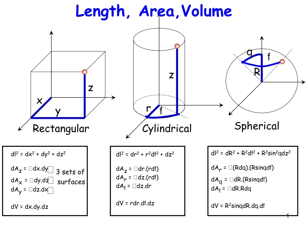
q f z R z x y r f Length, Area,Volume Spherical Rectangular Cylindrical dl2 = dR2 + R2df2 + R2sin2qdz2 dAr = (Rdq).(Rsinqdf) dAq= dR.(Rsinqdf) dAf = dR.Rdq dV = R2sinqdR.dq.df dl2 = dx2 + dy2 + dz2 dAz = dx.dy dAx= dy.dz dAy = dz.dx dV = dx.dy.dz dl2 = dr2 + r2df2 + dz2 dAz = dr.(rdf) dAr = dz.(rdf) dAf = dz.dr dV = rdr.df.dz 3 sets of surfaces
Vector Field Mapout local vectors at every point U (x,y,z)
Gradient In 1-D, it is dU/dx
dl = dU U . ^ ^ ^ dl = dx x + dy y + dz z dU(x,y,z) = ____ dx + ____ dy + _____ dz ∂U ∂y ∂U ∂z ∂U ∂x Gradient (Slope): U(x,y,z) = x ____ + y ____ + z _____ ∂U ∂z ∂U ∂x ∂U ∂y Gradient U U+dU
Connects divergence with flux: . B dv = B. dS Gauss’ Theorem = Closed Surface bounding a Volume (Divergence = Flux / volume)
.A(x,y,z) = ____ + ____ + _____ ∂Az ∂z ∂Ax ∂x ∂Ay ∂y Divergence Divergence (Outflow/Volume): [Jz(z+dz)-Jz(z)]dxdy = [∂Jz/∂z]dzdxdy = [∂Jz/∂z]dV Difference between opposite components gives net “outgoingness”
Connects curl with rotation: x B .dS = B. dl Stokes’ Theorem = Open Surface bounded by a Closed line (Curl = Rotation / volume)
∂Ay ∂x ∂Ax ∂y x A(x,y) = z ( ____ - ____ ) -Ax(x,y+dy) -Ay(x,y) Ay(x+dx,y) dy dx Ax(x,y) Curl Curl = Circulation/Area Difference between opposite components gives net rotation [Ax(x,y)-Ax(x,y+dy)]dx = [-∂Ax/∂y]dydx = [-∂Ax/∂y]dS
x A(x,y) = ^ ^ ^ x y z ∂/∂x ∂/∂y ∂/∂z Ax Ay Az Curl Curl = Circulation/Area
. . . - ∂Ax/∂y Visualizing the maths… CURL DIVERGENCE y y x x ∂Ax/∂x ∂Ay/∂x + ∂Ay/∂y + ∂Ax/∂y
Check ! Curl of Gradient = 0 Divergence of Curl = 0 . ( x A) = 0 x U = 0
∂2U ∂x2 ∂2U ∂y2 ∂2U ∂z2 2 U = _____ + _____ + ______ Slope of slope Curvature ! Laplacian Divergence of Gradient = 2 x ( x A) = (.A) - 2A Curl of Curl = Grad Div – Grad Squared
Relevance to electricity All these will be VERY relevant to future chapters !! (Curl and Div needed to define a vector) Static Electric fields have nonzero Divergence . E r No Curl x E = 0
Relevance to magnetism Static Magnetic fields have nonzero Curl x B J Zero Divergence .B = 0
Grad, Div, Curl in curvilinear coordinates Just as length, area and volume pick up funny pre-factors in curvilinear coordinates, so do Grad, Div and Curl. While there’s perhaps no point memorizing these (you have tables!), it’s worth knowing how they arise. We’ll take a quick look into this now
dl = h1dx1x1 + h2dx2x2 + h3dx3x3 U.dl = dU = Si(∂U/∂xi)dxi U = Si(∂U/∂xi)xi/hi ^ ^ ^ U = (∂U/∂r)r + (∂U/∂f)f/r + (∂U/∂z)z ^ ^ ^ U = (∂U/∂R)R + (∂U/∂q)q/R + (∂U/∂f)f/Rsinq Grad, Div, Curl in curvilinear coordinates
. B = B.dS/dV B1 h2h3dx2dx3 [ B1 h2h3 + ∂(B1h2h3)/∂x1.dx1 ] dx2dx3 . B = 1/(h1h2h3) x ∂(B1h2h3)/∂x1 + … Grad, Div, Curl in curvilinear coordinates dl = h1dx1x1 + h2dx2x2 + h3dx3x3
^ ^ ^ From slide 47, = r∂/∂r + (f/r)∂/∂f + z∂/∂z ^ ^ ^ Also, B = rBr + fBf + zBz A simple dot product would give .B = ∂Br/∂r + (1/r)∂Bf/∂f + ∂Bz/∂z But the correct divergence is .B = (1/r)∂(rBr)/∂r + (1/r)∂Bf/∂f + ∂Bz/∂z . B = 1/(h1h2h3) x ∂(B1h2h3)/∂x1 + … Grad, Div, Curl in curvilinear coordinates Note that you will see here that Divergence of B is NOT the dot product of grad with B !!!
A simple dot product would give .B = ∂Br/∂r + (1/r)∂Bf/∂f + ∂Bz/∂z dz df rdf But the correct divergence is .B = (1/r)∂(rBr)/∂r + (1/r)∂Bf/∂f + ∂Bz/∂z dr dr Grad, Div, Curl in curvilinear coordinates In cartesian, net outflow only if x component of B increases along x. But in curvilinear, the area itself increases along r !! This means even if B does not vary along r, the flux does!
( x B).dS = B.dl dl = dU U . . B = B.dS/dV Grad, Div, Curl in curvilinear coordinates So memorizing won’t help !!! Neither would trying to be too clever !!! Just need to go back to basics – the definitions of curl, div, grad – these you should remember
( x A).dS = A.dl - [A1h1 + ∂(A1h1)/∂x2.dx2]dx1 [A2h2 + ∂(A2h2)/∂x1.dx1]dx2 -A2h2dx2 A1h1dx1 /(h1h2h3) x2h2 ∂/∂x2 A2h2 x3h3 ∂/∂x3 A3h3 x1h1 ∂/∂x1 A1h1 x A = Grad, Div, Curl in curvilinear coordinates [∂(A2h2)/∂x1-∂(A1h1)/∂x2]/(h1h2)
( x A).dS = A.dl x1= r, x2 = f, x3 = z h1 = 1, h2 = r, h3 = 1 CYLINDRICAL x A = Grad, Div, Curl in curvilinear coordinates ^ ^ ^ r ∂/∂r Ar z ∂/∂z Az f r ∂/∂f Afr /r
( x A).dS = A.dl x1= R, x2 = q, x3 = f h1 = 1, h2 = R, h3 = Rsinq SPHERICAL Grad, Div, Curl in curvilinear coordinates ^ ^ ^ R ∂/∂R AR q R ∂/∂q AqR f Rsinq ∂/∂f AfRsinq /R2sinq x A =
2U = 1/(h1h2h3) x ∂[(h2h3/h1)∂U/∂x1]/∂x1 + … Combine Div. Grad Laplacian As an exercise, try writing 2 in spherical coordinates, and see if you can reproduce the expression on the inside cover at the back of the book
Summary • Saw how to add/subtract/multiply vectors • Easier to handle if we decompose into components • Decomposition can be done in various coordinate systems • Can convert between coordinates/unit vectors • Length, Area, Volume pick up ‘funny’ factors • Derivatives are Grad/Div/Curl, also acquire these factors