Download
1 / 44
440 likes | 459 Views
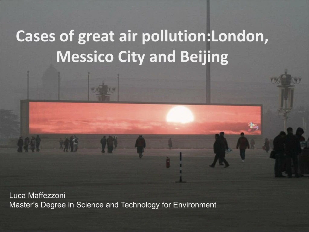
Cases of great air pollution:London, Messico City and Beijing. Luca Maffezzoni Master’s Degree in Science and Technology for Environment. Introduction.

E N D
Cases of great air pollution:London, Messico City and Beijing Luca Maffezzoni Master’s Degree in Science and Technology for Environment
Introduction • During the last 50 years, the cases of acute air pollution have increased exponentially, especially in big cities because of industrialization and the rise of strong highway traffic. • In this study, we will analyze three cases very relevant as the current ones in Mexico City ,Beijing and an historian event in the city of London. • Over the high pollutants emission, the others conditions necessary to have high concentration of pollutants are:1)Atmospheric stability, dry and low boundary layer height 2)City located in valleys with limited ventilation.
Particulate Matter Per la frazione PM10 l’efficienza del sistema di campionamento è del 55 % per dae = 10 µm mentre sì annulla per valori sopra i 15 µm La frazione PM2,5 è stata definita come quella porzione di particolato raccolta da un sistema di campionamento che ha un’efficienza del 48% per dae = 2.5µm mentre sì annulla per valori sopra i 4 µm • Among air pollutants, particulate matter(PM)has been found to be the most damaging to human health. • Especially the fine particles (PM2,5, particulate matter with an aerodinamyc diameter less than 2,5ug/m3) are associated with higher rates of mortality and morbidity under long-short term exposure. • Sources of particulate air pollution are of two types: • Primary sources: direct emission from natural and man-made particulate matter into the atmosphere. 2) Secondary sources: condensation of molecules present in the gaseous phase, which pass in the liquid or solid phase.
Chemical composition of PM • Inorganic Ions: sulfate (SO42-), nitrate (NO3-), ammonium (NH4 +) • Carbonaceous fraction: organic carbon (OC) and elemental carbon (EC) • Crustal material: (mineral dust: Si, Ca, Al, ...) + trace elements (Pb, Zn, ...) • H2O Average chemical composition of PM10 and PM2.5
Consequences and limits of PM • The World Health Organization, based on data collected in 2008, estimated that fine particles are responsible for approximately 2 million deaths per year worldwide. • In April 2008 the European Union has finally adopted a new directive (2008/50 / EC) for air quality limits. • The limits for the concentration of PM10 in the air shall be:-Maximum value for the annual average: 40 ug / m³ - Maximum daily (24-hour): 50 ug / m³ -Maximum number of exceedances allowed in a year: 35 • The annual average of PM 10 in the cities of the north of the italy is around 47ug/m3; outlaw!
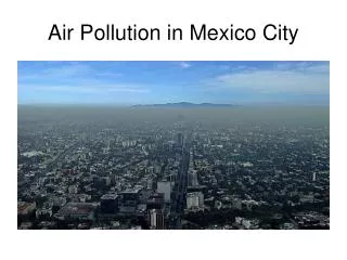
Mexico city • The valle de Mexico occupies 1300km2 • Elevation of 2240 meters above sea level • 20 milions of people live here • Bordered on the east and west by high mountain • dry weather and meteorological stability especially in winter • More than 30% of national industrial output is produced here • More than 3 milion of vehicles travels on its street daily
Campaign field • PM10 and PM2,5 ,precursor gas,meteorological measurement were taken in Mexico City • From February 23 to March 22 ,1997 • 6 sampling points in the core of the city • The goal of the project is understand concentration and chemical composition of the city PM.
PM10 measurements • The average 24-hr PM10 in core siteswas 75ug/m3 • The average concentrations at the boundary sites were about 30% less. • The U.S standard of 150ug/m3 was exceeded seven times • The maximum 24-hr concentration was 542ug/m3 • Dual peaks found at mid-morning and early evening
PM2,5 measurements • The average 24-hr concentrations was 36ug/m3. • The maximum 24-hr concentration was 184ug/m3 • The U.S standard of 65ug/m3 was exceeded four times during the study • The PM2,5 fraction generally comprised about 50% of PM10
Chemical measurement • Nitrate, ammonium and sulfate consituted approximately 15% of PM10 and 25% of PM2,5 • Valley-wide, carbon-containing aerosol accounted for about 30% of PM10 and 40% of PM2,5 • Geolofical material was the major contributor of PM10 around 50% • The highest concentrations of VOC was measured during morning hours • High levels of PAN were measured untill 30ppbV and they indicate the high organic oxidizing capacity.
Meteorological findings Because of the topographic setting of the city, the moderately strong insolation associated with its tropical latitude and high elevation, and weak prevailing synoptic winds, Mexico City is strongly affected by thermally and topographically induced circulation patterns. Three daytime flow patterns were observed during February and much of March. During the night the hight of BL decrease considerably.
Lethal London fog of 1952 • Situated into Tamigi’s Valley • 8 milions of people lived in London in 1952 • Long periods of High Pressure during Winter • Coal was the energy source most commonly used to heat homes • There were a lot of power plants and factories Causes of lethal fog from December 5 to December 9, 1952
PM and short-acute effects on mortality • Were measured only the air pollution concentrations of SO2 and TMS • during the event surpassed values of 4000ug/m3 for TMS and 0,3ppm for SO2 • For a 0.10-ppm increase in the previous day’s SO2 level, the estimated RR for daily mortality is 1.19. • Mortality remained double the normal for two weeks after the incident • During the week from 5-9 December the daily admissions increased of 164% mostly for cardiac and breathing problems.
Long-term Effects on mortality and morbidity • Total deaths from 1953 January 1 to march 31 were 8.635 more than the average but 1.328 for influence. • Deaths in January and February 1953 were 50% higher than expected • During the two weeks after the events respiratory and cardiac disease hospital admissions increased 163% • During and after the fog, emergency bed service applications increased, especially for respiratory and cardiac diseases.
CONSIDERATIONS • Air pollution level during the London fog of 1952 greatly exceeded WHO guidelines. • SO2 concentrations were 20 times higher • PM concentrations were about 5-19 times higher. • In london the episode was followed by high mortality rates for a period of 3 months. • Long-term mortality may also have been affected , as death rates did not return to normal levels until the end of february. • Air pollution in London of 1952 differs from modern pollution in its severity and pollutant mixture,because of the shift away from coal as a fuel source.
Beijing • Elevate concentrations of pollutants during all year • Megacity; population of >10 milions of inhabitants • Coal remains a major energy source in Beijing; • 27 milions of tons of coal provided more than 50%of total energy • The annual concentrations of PM10 from 2002 ranged between 141 and166ug/m3 and were three times the national standard of 50ug/m3 • Situated in a valley ,open on the south but bordered on the north,east,west by mountains. • Cold and dry winter; hot and cloudy summer
Population’s health and PM • Exposure–response functions are used in epidemiologic studies to link air pollution and its adverse health effects; • The Cox's proportional hazard model was often selected to determine the effect of air pollution on morbidity and mortality rates after adjusting for other factors such as cigarette smoking etc.. • The health adverse efforts of air pollution were calculated as: ∆E=E-Eo=Eoβ(C-Co)where β is the exposure–response coefficient, C and Co are the ambient and threshold pollutant concentrations and E and Eo are the health effects at C and Co, respectively. The ΔE or the health damage caused by increased pollution can be calculated if β, C, Co,and Eo are known. • The β values in this study are listed in this table
Health effects • The health impacts of PM pollution in 2002 may have been worse than in the other years because the PM10 concentration(166ug/m3)and the population are highest at that time. • In 2000 and 2001 the PM concentration is the same but effects were less than 2002 • In 2003 both concentration (141ug/m3)and the attributable number of cases were lower among 2000-2004. • The concentration in 2004 was close to 2003,but the estimated deaths due to PM was higher(23.733)cause increased population in the area
Economic costs of health effects • The value of statistical life(VOSL) concept was adopted to assess the health effects of PM pollution • It rappresents an individual’s willingness to pay(WTP)for a marginal reduction in the risk of dying. • For the valuation of reduced morbidity,besides WTP, the cost of illness(COI) approach could also be used • GDP is the common indicator that reflects the overall economic situation
The economic cost of health impacts of PM pollution in Beijing from 2000-2004 and the public welfare loss are shown in this table
Conclusions • To reduce the costs by air pollution in beijing, both the local and distant emissions should be well controlled • PM2,5 was more associated with premaure mortality than PM10 and his concentrations must be reduced urgently • Raw coal used in industrial plants could be replaced by cleaner sources such natural gas • Beijing government should preserve or restore bicycle lanes and provide free parking facilities to encourage the bicycle use
Transport pathways and potential sources of PM10 in Beijing • Investigated transport pathways and potential sources of PM10 in urban Beijing for all seasons over a continous 7-year data set from 2003 to 2009 by using multiple methods, including trajectory clustering,TSA end and PSCF. • The daily PM10 Air Pollution Index data were obtained from two rural sites, two suburban sites and eight urban sites • High PM10 concentrations in Beijing always occurred in the spring,followed by autumn and winter, than summer. • From 2000 to 2008 the average concentration of PM10 in beijing was 140ug/m3 with pick of 166ug/m3
Trajectory cluster and source locations • A two-stage clustering procedure was used to produce short and long source clustering.We obtain 9 clusters • Twelve 30° sectors were used to evaluate the influence of air mass direction on PM10 concentrations
Pathways:high concentration of PM10 • Southwest pathway:Based on cluster 9 occurred in april and october between summer and winter monsoon. The highest PM10 concentrations were probably associated with high emissions from Shanxi ,south of Hebei,Loess plateau and calm winds • South pathway:Based on cluster 8 was frequently occurred from may to september in association with the summer monsoon and topographic effects. High PM concentrations along this pathway were related to emission of industrial regions from this places.
The V-shapedsouthwestpathway:based on cluster 7 rapresentrelatively short and no-specialdirectionaltrajectroriesfromHebey and Shanxirelatedto the conversionofsummermonsoontowintermonsoon. The high frequencyofthispathway in septembercontributedto high concentrationsof PM in earlyautumn. • The northwestpathway:Based on cluster 1 and 3 frequentlyoccurreddurinautumnwinter and spring.The west-northwesterly flow thatcharacterizeclustershavebeenassociatedwith the mongolian High.Thispathwaypassedover the southof Mongolia and west ofinner Mongolia where the flowstransportsmineraldust and otherelements.
Pathways:low concentration of PM10 • The southeast pathway:Based on cluster 6, frequently occurred in june and july and may have been affected by summer monsoon. The high frequency of this relative clean pathway during june and july contributed to low concentrations in Beijing during young summer • The curved eastpathway: Based on cluster 5 occurred frequently in August and the flow may be asscociated with the summer monsoon. The frequency of occurence of this pathway peaked in August which corresponds to peak precipitations in Beijing direct consequence of low concentration.
The northern pathway:The northern pathway, including clusters 2 and 4 was the cleanest pathway. Airflows included in cluster 2 mainly traveled from the north,with the highest frequency in spring and a nearly in winter and autumn.Air masses of cluster 4 had the highest frequency in winter and spring too.Few anthropogenic PM10 sources were located on this pathway. Conclusions The results indicated that trajectories from the south and west were associated with high PM10 concentrations, while trajectories from the east and north were associated with relativerly low PM10 concentrations.The mean contribution of long distance transported PM10 in Beijing was about 39.3ug/m3 account for about 26% of the PM10 concentration in Beijing.
Seasonal-diurnal variations of PM2,5 in urban and rural sites in Beijing • High levels of PM2,5 in Beijing were associated to rapid grow of the city and the consequential increases in traffic and energy consumption. • The major sources of PM2,5 are dust, secondary aerosol, coal combustion, traffic exhaust and biomass burning. • PM2,5 has been misured continuosly from 2005-2007 in rural and urban sites.The goal of the study is to better understand the behavior of PM2,5 during the day and the seasons and the infuence of meteorological conditions. • Polluted air masses from urban areas and satellite towns of Beijing can be easily transported to SDZ by southwesterly winds, while relatively clean air masses arrive from other wind directions
Seasonal variations in PM2,5 concentrations • The climate was hot and humid in the summer, to cold and dry in the winter • The highest wind speeds occur during the spring ,medium in winter and lower in autumn and summer. • In the urban area, the highest PM2,5 concentrations generally occur during winter with an average of 115ug/m3. This is the results from a combination of increased emissions from heating sources and low boundary layer height. • In the rural area,the seasonal variation of PM2,5 differs from urban area.The concentrations are higher in spring and summer with an average of 75ug/m3 and lowest in winter. The dust produced by dust storms and wind erosion in the spring results in high PM2,5 concentrations during this season. The high summer concentrations may be caused for southerly winds that transported air pollutants from southern urban regions
The annualaverageswerealsocalculatedfrom 2005 to 2007 with a valuesof 86,5;93,5;84,4ug/m3 in urban site(BL) and 46;66,1;52,3ug/m3 in rural site(SDZ). • The higheraverage in 2006 is due tofrequentdustevents in thatspring. • The annualmeanof PM2,5 in bothsites are higherthan the valuesregistrated in Europe(6-25ug/m3) • The annualvariations in averagemonthly PM2,5concentrationsinrural site show similartrendsduring 2005-2007. The springmaximumisusuallyobserved in march-april ,the summermaximum in june-july and minimum in winter. • The yeartoyearvariabilityofmeteo-conditionsseemstohave no significantinfluence on seasonalpatternsof PM2,5 in rural site • In the urban area,seasonaltrendsappear more complex
Urban area variability • The winter maximum was reflected in the highest monthly averages in January 2006 and november 2005. • The rainfall in winter 2005 was two or four times higher than that seen in 2006-2007. • The highest average monthly PM2,5 concentration(114ug/m3)in summer appearing in june 2007, may be partially attributed to biomass burning in Beijing and surrounding region. Stable meteo-conditions in this month likely contribute as well. • The seasonal variability in urban area are mostly dominated by variability both emissions and meteo-conditions.
Diurnal variations in PM2,5 concentrations • Minimum PM2,5 concentrations appear afternoon at urban site with value of 77ug/m3but much earlier at rural site with a value of 45ug/m3. • Maxima of 102ug/m3 and 66ug/m3 occur at about 8-9 p.m at urban site and 1h earlier at rural site • The daily maximum for urban site appears in the early evening hours during both summer and winter, but in the summer, the morning peak is more pronunced and the evening peak has a lower amplitude than in winter. • The afternoon decrease of BL and wind speed companying with increased source activity during the afternoon rush hour results in the highest concentration during evening. • During the night although the BL is lowest, PM2,5 concentrations fall because of reductions in source activities and removal of particles by dry deposition. Average diurnal variations of PM2,5 Low meteo-influences
Meteo-conditions are important on diurnal variation in rural site • The minimum concentration is around 8:00 AM not in correlation with diurnal maximum of Bl which occurs around noon. • When the southeasterly winds shift to southwesterly wind after 11:00 AM the PM2,5 concentration shows a corresponding continuous increase until evening. The diurnal variations in PM2,5 in the rural area are significantly influenced by wind direction
Seasonal and diurnal variations of OC in PM2,5 and estimation of secondary OC in Beijing • Previous studies on the chemical compositions of PM2,5 in Beijing show that: • The annual average value is around 100ug/m3(milan=5ug/m3) • The carbonaceus species(EC+OC)constitute a major fraction of PM2,5 mass . • The secondary organic carbon(SOC) accounted for 25% to more than 50% of the total organic carbon on average • In this study were analized during one year: • The hourly OC concentrations • The hourly EC concentrations • Concentration of SOC and its contribution to OC
OC concentrations in PM2,5 in four seasons • In the case of OC there was an increasing trend in concentration from summer, to spring,to autumn to winter.On average,the OC concentrations in PM2,5 were 20ug/m3 in winter; 12ug/m3 in spring; 10ug/m3 in summer and 18ug/m3 in autumn. • The mean OC/EC ratios during the four seasons were 3.3; 2,6; 2,2; 2,2 in W,S,S,A. • The highest OC concentrations and OC/EC ratios in winter were mainly due to intensive emission of OC of coal burning during the heating period. • More than 70% of primary OC in Beijing is emitted from residential sources • OC/EC ratio from domestic coal burning can be ranging from 5 to 50. • OC/EC in industrial and transport sources are only from 0,4 to 6,1. • Less coal burnt in the other season: OC and OC/EC are lower.
Meteo-influence on seasonal variation • The industry and transport sectors accounted for nearly 30% of primary OC emissions in Beijing on annual average. OC sources of industrial and transport have no distinct seasonal changes, so the differences on OC among these seasons could be ascribed to the influence of weather condition • The OC concentration in autumn was higher than that in spring and summer.In spring and summer the OC concentrations became lower.The reason is that in spring the winds speed was much higher than in autumn, and in summer is the season of rainfall. • The highest concentration were in winter whit low BL and stagnants period.
Diurnal Variations of OC in PM2.5 • The EC concentration was generally higher during the nighttime than in the daytime, indicating the boundary layer depth plays an important role in the diurnal variation of atmospheric pollutants • In summer, the diurnal variations of EC were clearly but the OC concentration did not decrease in the afternoon
Additionaly OC in summer come from the solar radiation and photochemical oxidation ,strongest in the early afternoon,SOC could very likely contribute to this additional OC.(VOCs) • In spring, summer and autumn OC/EC ratios showed clear diurnal patterns, higher during the day but lower in the night. There may be two reasons related to this phenomenon,one is that the SOC is formed in day-time; the other is that a shift in OC and EC primary sources occurs between day and night. In fact during the night, whit the increased diesel emissions the averaged EC increased and OC/EC ratio be lower during night-time untill 6:00AM, cause particles of Diesel contain more EC. • When OC and EC are from primary emissions they have a god correlation, but not in summer cause there’s high presence of SOC.
Estimation of SOC • Eemitted owing to incomplete combustion of fossil fuel and biomass and is resistant to chemical reactions and useful to estimate the concentrations of POC and SOCC is predominatly. • Because primary OC/EC ratios are variable depending on the sources, is better to study the POC/EC ratio for day-time and night-time. • We just take the summer data as an example. • In these regression SCATTER-PLOT there aren’t rainy periods because it complicated the situation • The contribution of N in urban site is quite significant. N is the intercept of the regression line. OCpri = EC x (OC/EC)pri +N OCsec = OTtot-Ocpri N= contributions of POC from noncombustion sources
The SOC concentration was still present even during the night-time when the ozone concentration was quite lower than in day-time.The SOC night-time was considered to be a result of the accumulation of SOC formed in day-time and stagnant air at night. • Furthermore, night-time chemistry such as reactions of VOCs with nitrate radicals could also contribute to SOC formation at night. Since most of the secondary organic species originating from the oxidation of VOCs are semivolatile,the lower temperature and higher relative humidity in the night-time may partly contribute to increase the SOC concentration through the favorable partitioning in particle phase
Formation of SOC during high-ozone episode • Hourly concentration of NO was selected as the indicator of periods in which the oxidaton ability of the atmoshpere was weaker and local primary pollutants were dominant. • The estimated SOC concentrations and their fractions in OC also displayed inverse relationship with the NO concentration. These phenomena suggested that our estimate of the primary OC/EC ratio was reasonable and it can reflect well the periods when the photochemical oxidation was minimum and the primary sources of OC and EC were dominant. As the solar radiation strengthened in the late morning,the Ox concentrations increased and some volatile organic compounds could be oxidized to species with low vapor pressure and contributed to OC concentrations. These parts of OC were considered as SOC.
SOC concentrations in the four Seasons • The high SOC concentration in summer is mainly due to the enhanced photochemical activities in the season. In autumn,the averaged SOC concentrations were also higher compared to those in spring and winter. But its abundance in the total OC measured in autumn is smaller, only accounting for about 23% of the measured OC. The rather high absolute SOC contribution in autumn could be ascribed to the stagnated weather conditions favoring the formation and accumulation of secondary organic aerosols. • That is why the absolut SOC concentration in autumn was nearly the same as that in summer but the relative contribution of SOC to OC in aerosol in autumn was only the half of that in summer.
References Edgerton, S. A., Bian, X., Doran, J. C., Fast, J. D., Hubbe, J. M., Malone, E. L., ... & Ortiz, E. (1999). Particulate air pollution in Mexico City: A collaborative research project. Journal of the Air & Waste Management Association, 49(10), 1221-1229. Zhang, M., Song, Y., & Cai, X. (2007). A health-based assessment of particulate air pollution in urban areas of Beijing in 2000–2004. Science of the total environment, 376(1), 100-108. Yao, X., Lau, A. P., Fang, M., Chan, C. K., & Hu, M. (2003). Size distributions and formation of ionic species in atmospheric particulate pollutants in Beijing, China: 1—inorganic ions. Atmospheric Environment, 37(21), 2991-3000. Zhao, X., Zhang, X., Xu, X., Xu, J., Meng, W., & Pu, W. (2009). Seasonal and diurnal variations of ambient PM 2.5 concentration in urban and rural environments in Beijing. Atmospheric Environment, 43(18), 2893-2900. Zhu, L., Huang, X., Shi, H., Cai, X., & Song, Y. (2011). Transport pathways and potential sources of PM 10 in Beijing. Atmospheric Environment, 45(3), 594-604. Bell, M. L., & Davis, D. L. (2001). Reassessment of the lethal London fog of 1952: novel indicators of acute and chronic consequences of acute exposure to air pollution. Environmental health perspectives, 109(Suppl 3), 389.