Download
1 / 22
220 likes | 310 Views
Influence of solar wind density on ring current response. R.S. Weigel George Mason University. Geoeffectiveness – magnitude of a solar wind driver of geomagnetic activity Geoefficiency – amount of geomagnetic activity for a fixed magnitude of a solar wind driver. Output. Input.

E N D
Influence of solar wind density on ring current response R.S. Weigel George Mason University
Geoeffectiveness – magnitude of a solar wind driver of geomagnetic activity • Geoefficiency – amount of geomagnetic activity for a fixed magnitude of a solar wind driver
Output Input Efficiency=1 (unit change in input results in unit change output) 2x 2x
Output Input Efficiency=0 (unit change in input results in zero change output) 2x
More clarification Polar cap saturation is a classic example of geoefficiency. For low levels of interplanetary electric field vBs, the polar cap potential linearly increases with vBs. For high values it saturates. The geoeffective parameter is vBs. For high values, the geoeffective parameter is less geoeffective. Another way of thinking about geoeffective versus geoefficient is to consider an instrument with a temperature sensitivity. The output of the instrument depends on the ambient magnetic field. But for high temps, the output is less for a given input magnetic field. Temperature affects the geoefficiency. Temperature is not a driver in the traditional sense, but it does affect the output. (Technically, if you held the magnetic field constant and changed temperature, you would see a change in output, but physically, it is not usually cast in the system of equations as a driver, but rather a constant parameter that is slowly changing.
Mechanisms • Chen et al. [1994], Jordanova et al., [1998]and others– Simulations show ring current / Nps connection • Borovsky [1998] – Nsw pulses lead to response at geosynchronous; Thomson [1998] – Nps, Dst* correlation; Smith et al., [1999] – Dst has Nsw dependence that is independent of vBs at 3 hour time lag; O’Brien et al., [2000] – With more storms, no independent Dst dependence on Nsw • Lopez et al., [2004] – High compression ratio leads to higher reconnection rate • Boudouridis et al., [2005] – Dynamic pressure and geoefficiency of cross-polar-cap potential in event study • Lavraud et al. [2006] – CME and CIR storms had different epoch averages when CME or CIR was preceded by Bz>0
Approaches for computing geoefficiency • Linear filter model – Compute a linear filter (impulse response) model under different Nsw conditions. Efficiency is area under impulse response curve. • Integral ratios – Compare integrated input to integrated output for many events. Efficiency is slope computed using values of integrated output to integrated input for many events. • Epoch average ratio – Compute epoch averages first and then perform integral analysis on these curves. Efficiency is ratio of integrated epoch average of output to integrated epoch average input.
High Nsw Low Nsw Modeled -Dst for ht vBs t =
Result 1: Similar result if sorted by 4-hour running average of Nsw High Nsw Low Nsw Modeled -Dst for ht t =
Result 2: Similar result if sorted by Pdyn High Nsw Low Nsw Modeled -Dst for ht t =
Result 3: Nsw belongs in transfer function, not driver High Nsw Low Nsw Modeled -Dst for ht t =
h/ho Average Nsw [#/cc] hois geoefficiency at lowest Nsw value
High Nsw events (189) 5Nsw -Dst vBs/100 Low Nsw events (207) 5Nsw -Dst vBs/100
High Nsw events (189) 5Nsw -Dst vBs/100 Low Nsw events (207) 5Nsw -Dst vBs/100
h/ho Average Nsw [#/cc] hois geoefficiency at lowest Nsw value
Summary • Multiple approaches show geoefficiency depends on Nsw • Nsw should appear in transfer function, not coupling function • Geoefficiency differences most simply explained by Nsw rather than Pdyn • No significant difference (< 3% in RMS error) if more complex drivers are used • Epoch average method is least reliable