Download
1 / 60
600 likes | 606 Views
Control structure design: What should we measure, control and manipulate?. Sigurd Skogestad Department of Chemical Engineering NTNU, Trondheim. First African Control Conference, Cape Town, 04 December 2003. Outline. About myself Control structure design

E N D
Control structure design: What should we measure, control and manipulate? Sigurd Skogestad Department of Chemical Engineering NTNU, Trondheim First African Control Conference, Cape Town, 04 December 2003
Outline • About myself • Control structure design • A procedure for control structure design • Selection of primary controlled variables • Example stabilizing control: Anti slug control • Conclusion
Sigurd Skogestad • Born in 1955 • 1956-1961: Lived in South Africa (Durban & Johannesburg) • 1978: Siv.ing. Degree (MS) in Chemical Engineering from NTNU (NTH) • 1980-83: Process modeling group at the Norsk Hydro Research Center in Porsgrunn • 1983-87: Ph.D. student in Chemical Engineering at Caltech, Pasadena, USA. Thesis on “Robust distillation control”. Supervisor: Manfred Morari • 1987 - : Professor in Chemical Engineering at NTNU • Since 1994: Head of process systems engineering center in Trondheim (PROST) • Since 1999: Head of Department of Chemical Engineering • 1996: Book “Multivariable feedback control” (Wiley) • 2000,2003: Book “Prosessteknikk” (Tapir) • Group of about 10 Ph.D. students in the process control area
Research: Develop simple yet rigorous methods to solve problems of engineering significance. • Use of feedback as a tool to • reduce uncertainty (including robust control), • change the system dynamics (including stabilization; anti-slug control), • generally make the system more well-behaved (including self-optimizing control). • limitations on performance in linear systems (“controllability”), • control structure design and plantwide control, • interactions between process design and control, • distillation column design, control and dynamics. • Natural gas processes
Outline • About myself • Control structure design • A procedure for control structure design • Selection of primary controlled variables • Example stabilizing control: Anti slug control • Conclusion
Practice: Tennessee Eastman challenge problem (Downs, 1991)(“PID control”)
Control structure design • Not the tuning and behavior of each control loop, • But rather the control philosophy of the overall plant with emphasis on the structural decisions: • Selection of controlled variables (“outputs”) • Selection of manipulated variables (“inputs”) • Selection of (extra) measurements • Selection of control configuration (structure of overall controller that interconnects the controlled, manipulated and measured variables) • Selection of controller type (LQG, H-infinity, PID, decoupler, MPC etc.). • That is:Control structure design includes all the decisions we need make to get from ``PID control’’ to “Ph.D” control
Process control:Control structure design = plantwide control • Large systems • Each plant usually different – modeling expensive • Slow processes – no problem with computation time • Structural issues important • What to control? • Extra measurements • Pairing of loops
Control structure selection issues are identified as important also in other industries. Professor Gary Balas at ECC’03 about flight control at Boeing: The most important control issue has always been to select the right controlled variables --- no systematic tools used!
Process operation: Hierarchical structure RTO Need to define objectives and identify main issues for each layer MPC PID
Regulatory control (seconds) • Purpose: “Stabilize” the plant by controlling selected ‘’secondary’’ variables (y2) such that the plant does not drift too far away from its desired operation • Use simple single-loop PI(D) controllers • Status: Many loops poorly tuned • Most common setting: Kc=1, I=1 min (default) • Even wrong sign of gain Kc ….
Regulatory control……... • Trend: Can do better! Carefully go through plant and retune important loops using standardized tuning procedure • Exists many tuning rules, including Skogestad (SIMC) rules: • Kc = 0.5/k (1/) I = min (1, 8) • “Probably the best simple PID tuning rules in the world” • Outstanding structural issue: What loops to close, that is, which variables (y2) to control?
Supervisory control (minutes) • Purpose: Keep primary controlled variables (y1) at desired values, using as degrees of freedom the setpoints y2s for the regulatory layer. • Status: Many different “advanced” controllers, including feedforward, decouplers, overrides, cascades, selectors, Smith Predictors, etc. • Issues: • Which variables to control may change due to change of “active constraints” • Interactions and “pairing”
Supervisory control…... • Trend: Model predictive control (MPC) used as unifying tool. • Linear multivariable models with input constraints • Tuning (modelling) is time-consuming and expensive • Issue: When use MPC and when use simpler single-loop decentralized controllers ? • MPC is preferred if active constraints (“bottleneck”) change. • Avoids logic for reconfiguration of loops • Outstanding structural issue: • What primary variables y1 to control?
Local optimization (hour) • Purpose: Identify active constraints and possibly recompute optimal setpoints y1s for controlled variables • Status: Done manually by clever operators and engineers • Trend: Real-time optimization (RTO) based on detailed nonlinear steady-state model • Issues: • Optimization not reliable. • Modelling is time-consuming and expensive
Outline • About myself • Control structure design • A procedure for control structure design • Selection of primary controlled variables • Example stabilizing control: Anti slug control • Conclusion
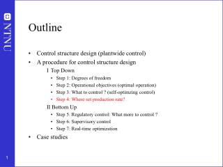
Stepwise procedure plantwide control I. TOP-DOWN Step 1. DEFN. OF OPERATIONAL OBJECTIVES Step 2. MANIPULATED VARIABLES and DEGREE OF FREEDOM ANALYSIS Step 3. WHAT TO CONTROL? (primary outputs, c= y1) Step 4. PRODUCTION RATE
II. BOTTOM-UP (structure control system): Step 5. REGULATORY CONTROL LAYER Stabilization and Local disturbance rejection What more to control? (secondary outputs y2) Step 6. SUPERVISORY CONTROL LAYER Decentralized control or MPC? Step 7. OPTIMIZATION LAYER (RTO)
Outline • About myself • Control structure design • A procedure for control structure design • Selection of primary controlled variables • Example stabilizing control: Anti slug control • Conclusion
y1 = c ? (economics) y2 = ? (“stabilization”) What should we control?
Optimal operation (economics) • Define scalar cost function J(u0,d) • u0: degrees of freedom • d: disturbances • Optimal operation for given d: minu0 J(u0,d) subject to: f(u0,d) = 0 g(u0,d) < 0
Active constraints • Optimal solution is usually at constraints, that is, most of the degrees of freedom are used to satisfy “active constraints”, g(u0,d) = 0 • Implementation of active constraints is usually simple. • We here concentrate on the remaining unconstrained degrees of freedom u.
Optimal operation Cost J Jopt uopt Independent variable u (remaining unconstrained)
Implementation: How do we deal with uncertainty? • 1. Disturbances d • 2. Implementation error n us = uopt(d*) – nominal optimization n u = us + n d Cost J Jopt(d)
Problem no. 1: Disturbance d d Cost J d* Jopt Loss with constant value for u uopt(d0) Independent variable u
Problem no. 2: Implementation error n Cost J d0 Loss due to implementation error for u Jopt us=uopt(d0) u = us + n Independent variable u
”Obvious” solution: Optimizing control Probem: Too complicated
Alternative: Look for another variable c to control Cost J Jopt copt Controlled variable c and keep at constant setpoint cs = copt(d*)
Self-optimizing Control • Define loss: • Self-optimizing Control • Self-optimizing control is when acceptable loss can be achieved using constant set points (cs)for the controlled variables c (without re-optimizing when disturbances occur).
Controlled variable: Feedback implementation Issue: What should we control?
Constant setpoint policy: Effect of disturbances (“problem 1”)
Effect of implementation error (“problem 2”) Good Good BAD
Self-optimizing Control – Illustrating Example • Optimal operation of Marathon runner, J=T • Any self-optimizing variable c (to control at constant setpoint)?
Self-optimizing Control – Illustrating Example • Optimal operation of Marathon runner, J=T • Any self-optimizing variable c (to control at constant setpoint)? • c1 = distance to leader of race • c2 = speed • c3 = heart rate • c4 = level of lactate in muscles
Further examples • Central bank. J = welfare. c=inflation rate • Cake baking. J = nice taste, c = Temperature • Biology. J = ?, c = regulatory mechanism • Business, J = profit. c = KPI = response time to order
Good controlled Variables c: Guidelines • Requirements for good candidate controlled variables (Skogestad & Postlethwaite, 1996): • Its optimal value copt(d) is insensitive to disturbances d (to avoid problem 1) • It should be easy to measure and control accurately (n small to avoid problem 1) • The variables c should be sensitive to change in inputs (to avoid problem 2) • The selected variables c should be independent (to avoid problem 2) • Rule: Maximize minimum singular value of scaled G • c = G u
Candidate controlled variables • Selected among available measurements y, • More generally: Find the optimal linear combination (matrix H):
Candidate Controlled Variables: Guidelines • Recall first requirement: Its optimal value copt(d) is insensitive to disturbances (to avoid problem 1) • Can we always find a variable combination c = H y which satisfies • YES!! Provided
Derivation of optimal combination (Alstad) • Starting point: Find optimal operation as a function of d: • uopt(d), yopt(d) • Linearize this relationship: yopt = F d • Look for a linear combination c = Hy which satisfies: copt = 0 • To achieve • Always possible if
Applications of self-optimizing control • Distillation • Tennessee Eastman Challenge problem • Power plant • +++
Outline • About myself • Control structure design • A procedure for control structure design • Selection of primary controlled variables • Example stabilizing control: Anti-slug control • Conclusion
Application: Anti-slug control Two-phase pipe flow (liquid and vapor) Slug (liquid) buildup
Slug cycle (stable limit cycle) Experiments performed by the Multiphase Laboratory, NTNU
z p2 p1 Experimental mini-loopValve opening (z) = 100%
z p2 p1 Experimental mini-loopValve opening (z) = 25%
z p2 p1 Experimental mini-loopValve opening (z) = 15%
z p2 p1 Experimental mini-loop:Bifurcation diagram No slug Valve opening z % Slugging
z p2 p1 Avoid slugging:1. Close valve (but increases pressure) No slugging when valve is closed Valve opening z %