Download

1 / 43
430 likes | 582 Views
Report Exemplar. Step 1: Purpose. State the purpose of your investigation. Pose an appropriate comparison investigative question and do not forget to include “by how much” . Explain why you are investigating this situation; G ive a brief background linked to research

E N D
Step 1: Purpose • State the purpose of your investigation. Pose an appropriate comparison investigative question and do not forget to include “by how much”. • Explainwhyyou are investigating this situation; • Give a brief background linked to research • Make a hypothesis – what you expect the outcome to be • Identify the variables you wish to investigate.
Your question must include • Variable that is being examined • Groups that are being compared • Population that inferences are being made about • Statistic (DIFFERENCE in sample median /mean)
Achieved The purpose of this investigation is to determine if the mean distance driven in a week (in kilometres) for males in the highest risk age group (15-24 years) is higher than the mean distance driven in a week (in kilometres) for females in the high risk age group and by how much from the sample of 206 crash statistics crashes where alcohol or drugs were recorded as a factorcommissioned by the New Zealand Ministry of Transport in 2011. • The difference in sample means between male and female drivers from this sample will be used to make a formal inference about the 1409 serious or minor crashes where alcohol or drugs were recorded by the New Zealand Ministry of Transport as a factor in 2011.
Merit I am interested in this investigation as the reason for more males being involved in crashes than females is often given as “males drive much more than females”. It is my belief that, on average, males will have driven further than females.
Excellence This belief is supported by research carried out by the New Zealand Ministry of Transport who claim that “on average, men drive just over 12,000 km per driver per year, while women average just over 8,000 km per driver per year.” However, “Work-related travel accounts for nearly one third of all household driving time and distance.” (Ministry of Transport, 2011)
Second investigation Question In a study released by Quality Planning, an analytics company, based in San Francisco, that validates policyholder information for auto insurers found that “men break more traffic laws and drive more dangerously than women. Because they violate laws designed to make the roads safer, men cause more accidents and expensive damage.” This suggests that it might also be interesting to investigate by how much the mean insurance claim (in $) for males is higher than the mean insurance claim (in $) for females for those involved in crashes in the same 2011 study commissioned by the New Zealand Ministry of Transport.
Research integrated into the question Dr. Raj Bhat, president of Quality Planning, claims that men have about 5% more violations that result in accidents than women and because “men are also more likely to violate laws for speeding, passing, and yielding, the resulting accidents caused by men lead to more expensive claims than those caused by women." These statistics are based on an American study and may not apply in New Zealand but my feeling is that it will also be true in New Zealand.
List references as you go- clean them up at the end • http://www.transport.govt.nz/research/Documents/Driver travel-March 2012.pdf • New Zealand Household Travel Survey 2008– 2011, Downloaded 13/5/13 Men Break More Traffic Laws, Drive More Dangerously Than Women, Concludes QPC Study 11/13/2008, http://www.qualityplanning.com/
Data Source • The study has been motivated by recent popular media campaigns by the New Zealand Transport Association. http://www.nzta.govt.nz/about/advertising/drink-driving/legend.html
Information about the data In 2011, there were 1409 serious or minor crashes where alcohol or drugs were recorded as a factor. A random sample was taken from these drivers and they were interviewed in person by researchers. The data obtained is what I will be analysing in my assignment.
Achieved: • Dot plots and box and whisker plots are produced and summary statistics, including the difference between the sample means/medians, have been calculated.
Sample distributions- Achieved • The sample distributions are discussed and compared in context. This could involve • Comparing the shift/centre • Spread • Shape • Unusual features • Summary statistics
Sample distributions: Merit • As for Achieved with links to the population or investigative question.
Sample distributions: Excellence • As for Merit with explanations for the features of the data and the impact of these on the context or question. Relevant reference to the research.
To avoid cumbersome wording.. Male distance refers to the distance driven in a week (in kilometres) for males in the highest risk age group (15-24 years) in crashes where alcohol or drugs were recorded as a factorcommissioned by the New Zealand Ministry of Transport in 2011. Similarly I will refer to female distance in the same study. Population refers to the 1409 serious or minor crashes where alcohol or drugs were recorded in 2011 by the Ministry of Transport.
Initial Visual Interpretation My initial visual impression is that the median of male distance is similar to the median female distance. This is not what I predicted.
Comparing the shift/centre In the samples, I found that the female distance was 116.6 km and that male distance was 110.4 km.
Comparing the shift/centre- add comment The result is quite surprising as I thought the male distance would be higher.
Comparing the shift/centre- add comment The difference between these values is quite small (6.2km).
Comparing the shift/centre- relate to the population Considering that the information was obtained in an interview and those interviewed would have to estimate these values, we cannot be sure that this result would be the same as the population.
Comparing the shift/centre- relate to the population The distribution of the data suggests that people may have been inclined to round their estimates to the nearest 10 km.
Comparing the shift/centre- add research This result is also contrary to my research (Ministry of Transport, 2011) which indicated male distance was greater than female distance. This research however included all driving rather than just driving under the influence of drugs or alcohol.
Comparing the shape The distribution of the male distance driven in a week appears to be skewed to the right. The bulk of sample data for males is between 20 and 180 kilometres. The maximum value is 263 km.
Comparing the shape The distribution of the female distance driven in a week is skewed to the right. The bulk of sample data for females is between 10 and 160 kilometres. The rest is spread out to a maximum of 263 km.
Comparing the spread The middle 50% of male distance is between 82.5 km and 140.5 km- an interquartile range of 58 km. The middle 50% of female distance is between 78.5 km and 140.5 km- an interquartile range of 66 km.
Comparing the spread As the boxes overlap, I am not happy to make a call that the female distance is higher than the male distance. Also, as this is only one sample from the population, I would expect to get a different but similar result if I were to take another sample.
Personal comment explaining the spread As this age group would generally be single, it is likely that females and males would have similar driving habits i.e. driving distances to school or work would be similar.
Refer to the population As the sample size in each category is reasonable (87 for female distance and 119 for male distance), I would be confident that the comparisons would be similar in the population.
Shift/overlap As the box for female distance overlaps the box for male distance, I would be confident to say that there is no significant difference between the medians or means of the groups.To test this I will calculate a bootstrapping confidence interval to obtain a measure of the difference between the means of the two groups. A bootstrap confidence interval is a range of believable values for the difference in means of the male distance and female distance.
The formal inference used was a bootstrap confidence interval (-0.50 mmHg, 3.30mmHg) of the sample differences between the male and female SBP. The call cannot be made that back in the population of British male and females consuming a high fat diet there is a difference between British male and female SBP.