Download
1 / 47
530 likes | 1.19k Views
10. Laplace TransforM Technique. CIRCUITS by Ulaby & Maharbiz. Overview. Analysis Techniques. Circuit Excitation Method of Solution Chapters 1. dc (w/ switches) Transient analysis 5 & 6 2. ac Phasor -domain analysis 7 -9

E N D
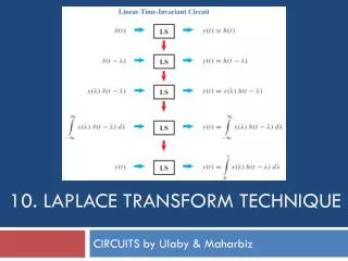
10. Laplace TransforM Technique CIRCUITS by Ulaby & Maharbiz
Analysis Techniques Circuit Excitation Method of Solution Chapters 1. dc (w/ switches) Transient analysis 5 & 6 2. ac Phasor-domain analysis 7 -9 ( steady state only) 3. any waveform Laplace Transform This Chapter (single-sided) (transient + steady state) 4. Any waveform Fourier Transform 11 (double-sided) (transient + steady state) Single-sided: defined over [0,∞] Double-sided: defined over [−∞,∞]
Singularity Functions A singularity function is a function that either itself is not finite everywhere or one (or more) of its derivatives is (are) not finite everywhere. Unit Step Function
Singularity Functions (cont.) Unit Impulse Function For any function f(t):
Laplace Transform of Singularity Functions For A = 1 and T = 0:
Laplace Transform of Delta Function For A = 1 and T = 0:
Properties of Laplace Transform 1. Time Scaling Example 2. Time Shift
Properties of Laplace Transform (cont.) 3. Frequency Shift Example 4. Time Differentiation
Properties of Laplace Transform (cont.) 5. Time Integration 6. Initial and Final-Value Theorems
Properties of Laplace Transform (cont.) 7. Frequency Differentiation 8. Frequency Integration
Partial Fraction Expansion Partial fraction expansion facilitates inversion of the final s-domain expression for the variable of interest back to the time domain. The goal is to cast the expression as the sum of terms, each of which has an analog in Table 10-2. Example
1. Partial FractionsDistinct Real Poles Example The poles of F(s) are s= 0,s= −1, ands= −3. All three poles are real and distinct.
Example 2. Partial FractionsRepeated Real Poles Cont.
2. Partial FractionsRepeated Real Poles Example cont.
3. Distinct Complex Poles • Procedure similar to “Distinct Real Poles,” but with complex values for s • Complex poles always appear in conjugate pairs • Expansion coefficients of conjugate poles are conjugate pairs themselves Example Note that B2 is the complex conjugate of B1.
3. Distinct Complex Poles (Cont.) Next, we combine the last two terms:
4. Repeated Complex Poles: Same procedure as for repeated real poles
Property #3a in Table 10-2: Hence:
s-Domain Circuit Models Under zero initial conditions:
Example 10-11: Interrupted Voltage Source Initial conditions: Voltage Source (s-domain) Cont.
Transfer Function In thes-domain, the circuit is characterized by a transfer function H(s), defined as the ratio of the outputY(s)to the inputX(s),assuming that all initial conditions relating to currents and voltages in the circuit are zero at t = 0−.
Transfer Function (cont.) Convolution in time domain Multiplication in s-domain
Convolution IntegralImpulse Response h(t): output of linear system when input is a delta function Output Input y(t) cannot depend on excitations occurring after time t Assumes x(t) = 0 for t < 0 Definition of convolution
Convolution Integral • Can be used to determine output response entirely in the time domain • Can be useful when input is a sequence of experimental data or not a function with a definable Laplace transform • Convolution can be performed by shifting h(t) or x(t): h(t) shifted x(t) shifted
Integral can be computed graphically at successive values of t.
0.86 @1s 0.11@ 2s