Download

1 / 14
160 likes | 722 Views
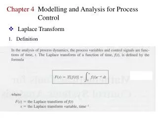
Laplace Transform. Forward Laplace Transform. Decompose a signal f ( t ) into complex sinusoids of the form e s t where s is complex: s = s + j 2 p f Forward (bilateral) Laplace transform f ( t ): complex-valued function of a real variable t

E N D
Forward Laplace Transform • Decompose a signal f(t) into complex sinusoids of the form es t where s is complex: s = s + j2pf • Forward (bilateral) Laplace transform f(t): complex-valued function of a real variable t F(s): complex-valued function of a complex variable s • Bilateral means that the extent of f(t) can be infinite in both the positivet and negativet direction (a.k.a. two-sided)
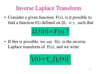
Inverse (Bilateral) Transform • Inverse (Bilateral) Transform is a contour integral which represents integration over a complex region– recall that s is complex c is a real constant chosen to ensure convergence of the integral • Notation F(s) = L{f(t)} variable t implied for L f(t) = L-1{F(s)} variable s implied for L-1
f(t) L F(s) Laplace Transform Properties • Linear or nonlinear? • Linear operator
Laplace Transform Properties • Time-varying or time-invariant? This is an odd question to ask because the output is in a different domain than the input.
Convergence • The condition Re{s} > -Re{a} is the region of convergence, which is the region of s for which the Laplace transform integral converges • Re{s} = -Re{a} is not allowed (see next slide)
Im{s} f(t) 1 t Re{s} f(t) = e-a t u(t) causal Re{s} = -Re{a} Regions of Convergence • What happens to F(s) = 1/(s+a) at s = -a? (1/0) • -e-a t u(-t) and e-a t u(t) have same transform function but different regions of convergence f(t) t -1 f(t) = -e- a t u(-t) anti-causal
Review of 0- and 0+ • d(t) not defined at t = 0 but has unit area at t = 0 • 0- refers to an infinitesimally small time before 0 • 0+ refers to an infinitesimally small time after 0
Unilateral Laplace Transform • Forward transform: lower limit of integration is 0- (i.e. just before 0) to avoid ambiguity that may arise if f(t) contains an impulse at origin • Unilateral Laplace transform has no ambiguity in inverse transforms because causal inverse is always taken: No need to specify a region of convergence Disadvantage is that it cannot be used to analyze noncausal systems or noncausal inputs
As long as e-s t decays at a faster rate than rate f(t) explodes, Laplace transform converges for some M and s0,there exists s0 > s to make the Laplace transform integral finite We cannot always do this, e.g. does not have a Laplace transform Existence of Laplace Transform
Fourier vs. Laplace Transform Pairs Assuming that Re{a} > 0