PRAM Submodels and Assumptions

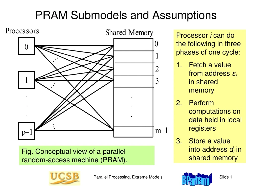
1. PRAM Submodels and Assumptions • Processor i can do • the following in three • phases of one cycle: • Fetch a value from address si in shared memory • Perform computations on data held in local registers • 3. Store a value into address di in shared memory Fig. Conceptual view of a parallel random-access machine (PRAM). Parallel Processing, Extreme Models

2. Types of PRAM Fig. Submodels of the PRAM model. Parallel Processing, Extreme Models

3. Types of CRCW PRAM CRCW submodels are distinguished by the way they treat multiple writes: Undefined: The value written is undefined (CRCW-U) Detecting: A special code for “detected collision” is written (CRCW-D) Common: Allowed only if they all store the same value (CRCW-C) [This is sometimes called the consistent-write submodel ] Random: The value is randomly chosen from those offered (CRCW-R) Priority: The processor with the lowest index succeeds (CRCW-P) Max/Min: The largest/smallest of the values is written (CRCW-M) Reduction: The arithmetic sum (CRCW-S), logical AND (CRCW-A), logical XOR (CRCW-X), or another combination of values is written Parallel Processing, Extreme Models

4. Implications of the CRCW Hierarchy of Submodels EREW < CREW < CRCW-D < CRCW-C < CRCW-R < CRCW-P A p-processor CRCW-P (priority) PRAM can be simulated (emulated) by a p-processor EREW PRAM with slowdown factor Q(log p). Our most powerful PRAM CRCW submodel can be emulated by the least powerful submodel with logarithmic slowdown Efficient parallel algorithms have polylogarithmic running times Running time still polylogarithmic after slowdown due to emulation We need not be too concerned with the CRCW submodel used Simply use whichever submodel is most natural or convenient Parallel Processing, Extreme Models

5. Some Elementary PRAM Computations p elements Initializing an n-vector (base address = B) to all 0s: for_proc i = 0 to p-1 do for j = 0 to n/p – 1 do if jp + i < n then M[B + jp + i] := 0 endfor endfor n/p segments Adding two n-vectors and storing the results in a third (base addresses A, B, C) [C+ jp + i] := [A+ jp + i] + [B+ jp + i] Parallel Processing, Extreme Models

6. Fig. EREW PRAM data broadcasting without redundant copying. Data Broadcasting Making p copies of B[0] by recursive doubling for k = 0 to log2p – 1 do for_proc j = 0 to p-1 do copy B[j] into B[j + 2k] endfor endfor Fig. Data broadcasting in EREW PRAM via recursive doubling. Can modify the algorithm so that redundant copying does not occur and array bound is not exceeded Parallel Processing, Extreme Models

7. All-to-All Broadcasting on EREW PRAM EREW PRAM algorithm for all-to-all broadcasting for_proc j = 0 to p-1 do write own data value into B[j] endfor for_proc j = 0 to p-1 do for k = 1 to p – 1 do Read the data value in B[(j + k) mod p] endfor endfor 0 j p – 1 This O(p)-step algorithm is time-optimal Parallel Processing, Extreme Models

8. Sorting on PRAM Naive EREW PRAM sorting algorithm (using all-to-all broadcasting) for_proc j = 0 to p-1 do write 0 into R[ j ] endfor for_proc j = 0 to p-1 do for k = 1 to p – 1 do l := (j + k) mod p if S[ l ] < S[ j ] or S[ l ] = S[ j ] and l < j then R[ j ] := R[ j ] + 1 endif endfor endfor for_proc j = 0 to p-1 do write S[ j ] into S[R[ j ]] endfor This O(p)-step sorting algorithm is far from optimal; sorting is possible in O(log p) time Parallel Processing, Extreme Models

9. Parallel Prefix Computation Fig. Parallel prefix computation in EREW PRAM via recursive doubling. Parallel Processing, Extreme Models

10. Parallel Prefix Computation EREW PRAM parallel prefix computation algorithm for_proc j = 0 to p-1 do copy X[j] into S[j] endfor s := 1 while s < p do for_proc j = 0 top – s-1 do S[j + s] := S[j] S[j + s] endfor s := 2s endwhile Broadcast S[p – 1] to all processors (if needed) speedup = O(p/log p) Parallel Processing, Extreme Models

11. PRAM Matrix Multiplication with m2 Processors PRAM matrix multiplication using m2 processors for_proc (i, j), 0 i, j < m, do begin t := 0 for k = 0 to m – 1 do t := t + aikbkj endfor cij := t end endfor Processors are numbered (i, j), instead of 0 to m2 – 1 Q(m) steps: Time-optimal A B C Fig. PRAM matrix multiplication; p = m2 processors. Parallel Processing, Extreme Models

12. PRAM Matrix Multiplication with m Processors PRAM matrix multiplication using m processors for_proc i = 0 tom-1 do for j = 0 to m–1 do t := 0 for k = 0 to m–1 do t := t + aikbkj endfor cij := t endfor endfor Q(m2) steps: Time-optimal C A B Parallel Processing, Extreme Models

13. PRAM Matrix Multiplication with Fewer Processors Algorithm is similar, except that each processor is in charge of computing m/p rows of C Q(m3/p) steps: Time-optimal A B C Parallel Processing, Extreme Models

14. Some Implementation Aspects This section has been expanded; it will eventually become a separate chapter Options: Crossbar Bus(es) MIN Bottleneck Complex Expensive Fig. A parallel processor with global (shared) memory. Parallel Processing, Extreme Models

15. P0 P1 P2 P3 P4 P5 P6 P7 M0 M1 M2 M3 M4 M5 M6 M7 An 8  8 crossbar switch Processor-to-Memory Network Crossbar switches offer full permutation capability (they are nonblocking), but are complex and expensive: O(p2) Even with a permutation network, full PRAM functionality is not realized: two processors cannot access different addresses in the same memory module Practical processor-to-memory networks cannot realize all permutations (they are blocking) Parallel Processing, Extreme Models

16. Removing the Processor-to-Memory Bottleneck Challenge: Cache coherence Fig. A parallel processor with global memory and processor caches. Parallel Processing, Extreme Models

17. Distributed Shared Memory Fig. A parallel processor with distributed memory. Parallel Processing, Extreme Models

18. Multistage Interconnection Networks Numerous indirect or multistage interconnection networks (MINs) have been proposed for, or used in, parallel computers They differ in topological, performance, robustness, and realizability attributes We have already seen the butterfly, hierarchical bus, beneš, and ADM networks Fig. The sea of indirect interconnection networks. Parallel Processing, Extreme Models

19. Butterfly Processor-to-Memory Network Not a full permutation network (e.g., processor 0 cannot be connected to memory bank 2 alongside the two connections shown) Is self-routing: i.e., the bank address determines the route A request going to memory bank 3 (0 0 1 1) is routed: lower upper upper Fig. Example of a multistage memory access network. Parallel Processing, Extreme Models

20. Butterfly as Multistage Interconnection Network Fig. Butterfly network used to connect modules that are on the same side Fig. Example of a multistage memory access network Generalization of the butterfly network High-radix or m-ary butterfly, built of mm switches Has mq rows and q + 1 columns Parallel Processing, Extreme Models

21. Beneš Network Fig. Beneš network formed from two back-to-back butterflies. A 2q-row Beneš network: Can route any 2q 2q permutation It is “rearrangeable” Parallel Processing, Extreme Models

22. Routing Paths in a Beneš Network Fig. Another example of a Beneš network. Parallel Processing, Extreme Models

23. Fig. Example of sorting on a binary radix sort network. Self-Routing Permutation Networks Do there exist self-routing permutation networks? (The butterfly network is self-routing, but it is not a permutation network) Permutation routing through a MIN is the same problem as sorting Parallel Processing, Extreme Models

24. Parallel Processing, Extreme Models