Download

1 / 47
480 likes | 743 Views
Magnetic Resonance Imaging. Dr Sarah Wayte University Hospital of Coventry & Warwickshire. GE MR Scanner. Receiver Coils. ‘Typical’ MR Examination. Surface coil selected and positioned Inside scanner for 20-30min Series of images in different orientations & with different contrast obtained

E N D
Magnetic Resonance Imaging Dr Sarah Wayte University Hospital of Coventry & Warwickshire
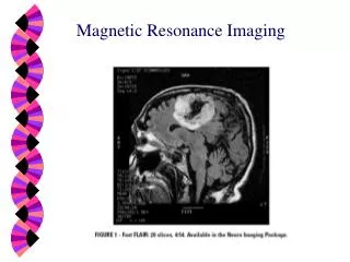
‘Typical’ MR Examination • Surface coil selected and positioned • Inside scanner for 20-30min • Series of images in different orientations & with different contrast obtained • It is very noisy
What is so great about MRI? • By changing imaging parameters (TR and TE times) can alter the contrast of the images • Can image easily in ANY plane (axial/sag/coronal) or anywhere in between
Spatial Resolution • In slice resolution = Field of view / Matrix • Field of view typically 250mm head • Typical matrix 256 • In slice resolution ~ 0.98mm • Slice thickness typically 3 to 5 mm • High resolution image • FOV=250mm, 512 matrix, in slice res~0.5mm • Slice thickness 0.5 to 1mm
Any Plane • Magnetic field varied linearly from head to toe • Hydrogen nuclei at various frequency from head to toe (ωo=γBo) • RF pulse at ωo gives slice through nose (resonance) • RF pulse at ωo+ ωgives slice through eye RF wave ωo+ωωoωo - ω Slice selection gradient
Sagittal/Coronal Plane • Sagittal slice: vary gradient left to right • Coronal slice: apply vary gradient anterior to posterior • Combination of sag & coronal gradient can give any angle between
Image Contrast TR=525ms TE=15ms TR=2500ms TE=85ms
Image Contrast • Depends on the pulse sequence timings used (TR/TE) • 3 main types of contrast • T1 weighted • T2 weighted • Proton density weighted • Explain for 90 degree RF pulses
TR and TE • To form an image have to apply a series of 90o pulses (eg 256) and detect 256 signals • TR = Repetition Time = time between 90o RF pulses • TE= Echo Time = time between 90o pulse and signal detection TR TR 90-----Signal-------------90-----Signal-----------90-----Signal TE TE TE
Bloch Equation • Bloch Equations BETWEEN 90o RF pulses Signal=Mo[1-exp(-TR/T1)] exp(-TE/T2) • TR<T1, TE<<T2, T1 weighted • TR~3T1, TE<T2, T2 weighted • TR~3T1, TE<<T2, Mo or proton density weighted TR TR 90-----Signal-------------90-----Signal-----------90-----Signal TE TE TE
T1 weighted Water dark Short TR=500ms Short TE<30ms T2 weighted Water bright Long TR=1500ms (3xT1max) Long TE>80ms PD/T1/T2 Weighted Image PD weighted • Long TR=1500ms (3xT1max) • Short TE<30ms
T1/T2 Weighted Image TR = 562ms TE = 20ms TR = 4000ms TE = 132ms
T1/T2 Weighted TR=525ms TE=15ms TR=2500ms TE=85ms
Proton Density/T2 TR = 3070ms TE = 15ms TR = 3070ms TE = 92ms
Proton Density/T2 TR = 3070ms TE = 15ms TR = 3070ms TE = 92ms
Lumbar Spine ImagesDisc protrusion L5/S1. Degenerative changes bone.
Imaging Time (Spin Warp) • 1 line of image (in k-space) per TR Imaging time = TR x matrix x Repetitions • Reps typically 2 or 4 (improves SNR) • E.g. TR=0.5s, Matrix=256, Reps=2 Image time = 256s = 4min 16s • During TR image other slices • Max no slices = TR/TE • e.g. 500/20=25 or 2500/120=21
Speeding Things Up 1 • Spin warp T2 weighted image, 256 matrix, 3.5s TR, 2reps • Imaging time = 3.5 x 256 x 2 ~ 30min!!! • Solution: acquire 21 lines k-space per 90o pulse
Speeding Things Up 2 • With 21 signals per 90o pulse for 256 matrix, 3.5s TR, 2reps Imaging time = 3.5 x 256 x 2/21 ~ 1min 25s • All images I’ve shown so far use this technique (Fast spin echo or turbo spin echo)
Even Faster Imaging • How fast? 14-20 images in a breath-hold (30 images @ 3T) • Use < 90 degree flip (α) • Some Mz magnetisation remains to form the next image, so TR<20ms • Drawback- less magnetisation/signal in transverse plane Mz Signal = MoCosα
T1 Breath-hold Images 14 slices in 23s breath-hold (t1_fl2d_tra_bh) TR=16.6ms, TE=6ms α=70o
T2 breath-hold images 19 slice in 25s breath-hold (t2-trufi_tra_bh) TR=4.3ms TE=2.1ms α=80o
Echo Planar Imaging Takes TSE/FSE to the extreme by acquiring 64 or 128 image lines (signals) following a single 90 degree RF pulse Image matrix size (64)2 or (128)2 (poor resolution)
EPI Imaging • Each slice acquired in 10s of milliseconds • Lower resolution • More artefacts www.ph.surrey.ac.uk
EPI Imaging • Each slice acquired in ~10ms • Used as basis for functional MRI (fMRI) • Images acquired during ‘activation’ (e.g. finger tapping) and rest. Sum active and rest and subtract Right motor cortex excited with left finger tapping, in close proximity with tumour www.icr.chmcc.org
Functional MRI (fMRI) • Concentration of oxyhaemoglobin brighter (longer T2* than de-oxyhaemoglobin) Subtracted image of bright ‘dots’ of activated brain • Super-impose dot image over ‘anatomical’ MR image fMRI of patient with tumour near right motor cortex Active area with left finger tapping Shows right motor cortex close too, but not overlapping tumour www.ich.ucl.ac.uk
Imaging Blood Flow • Apply series of high flip angle pulses very quickly (short TR) • Stationary tissue does NOT have time to recover, becomes saturated • Flowing blood, seen no previous RF pulses, high signal from spins each time Flip Flip TR
MRA Base Images • 72 slices through head • Brain tissue ‘saturated’ high signal from moving blood • Processed by computer to produce Maximum Intensity Projections (MIPs) • Maximum signal along line of site displayed
Diffusion Imaging • Uses EPI imaging technique with additional bi-polar gradients in x, y & z directions • Bi-polar gradients also varied in amplitude • No diffusion – high signal • More diffusion- lower signal
Different Amp Diffusion Gradient: Ischemic Stroke? Stroke reduces diffusion Bright on diffusion weighted image Amp = 0 Amp = 500 Amp = 1000
Diffusion Co-efficient Map & Images Diffusion co-efficient map Diffusion image Intensity α 1/Diffusion (& T2) Intensity α Diffusion Co-efficient
Anisotropic Diffusion Diffusion gradient Diffusion gradient
Anisotropic Diffusion: Diffusion tensor imaging • Anisotropic diffusion in white matter tracks • Apply diffusion gradients in 12-15 direction • ‘Track’ white matter track direction by diffusion anisotropy Brainimaging.waisman.wisc.edu www.cimst.ethz.ch