Download
1 / 22
220 likes | 404 Views
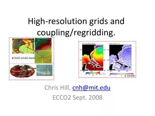
High-resolution grids and coupling/ regridding . ECCO2 cs510 mesh. Chris Hill, cnh@mit.edu ECCO2 Sept. 2008. D. Chelton. High-res horizontal grid strategy. Sticking with orthogonal curvilinear grid? High-order numerics cleaner. OS7MP etc… Grid generation more challenging.

E N D
High-resolution grids and coupling/regridding. ECCO2 cs510 mesh Chris Hill, cnh@mit.edu ECCO2 Sept. 2008 D. Chelton
High-res horizontal grid strategy • Sticking with orthogonal curvilinear grid? • High-order numerics cleaner. OS7MP etc… • Grid generation more challenging. • For now, targeting orthogonal, but maybe should look more closely at trade offs (cf Putnam and Lin). • Numerical generation is (much) harder • Grid can be hard to control • But we think we understand numerics • Targeting base grid at very high-resolution that can be “cleanly” coarsened (and can be used globally or regionally). Largest number of common integer factors – (degrees, minutes, seconds are really useful) 510 – 16 factors, 512 – 10 factors, 360 – 24 factors, 4320 – 48 factors. Grid spacing should reflect deformation radius. Highest res should resolve e.g. ∆ < 2km @ f~10-4s†. Better treatment of polar regions, quasi-isotropic grid spacing in high-latitudes – next slides.
Avoiding converging meridians in Antarctic 70S 65W Lat-lon to 57N
Compatible Polar Cap “Isotropic” Arctic 57N ~63N Lat-lon to 70S 38W, 67.5N
Compatible grid hierarchy Requirements – large number of factors and grid lines at 65W, 38W, 38W+90, 38W+180, 38W+270 18 levels of refinement ranging from 17280 – 80 points around globe. …. all we need is a foundation, general curvilinear 17280 point polar-cap and Antarctic split grid
Generating high-res Arctic and Antarctic grids. • Two existing grid generation tools for MITgcm. Initial plan was to use these, however: • Standard cube-sphere generating code (J Purser code) based on hard coded, high-order numerical solution to analytic conformal map (angle preserving) of unit circle to unit square. Not good for general grid generation, but very accurate. • Spgrid (E Hill code) solves elliptic problem on a sphere for a somewhat irregular domain, but • Has accuracy issues for large problem sizes. • Region boundaries cannot be arbitrary curves. Precludes “recursive” approach to handling large problem size. • Has occasional orthogonality issues. • Coded for sphere. • Neither of two approaches can create accurate grids with complete flexibility. • New tool based on “conformal mapping” of arbitrary two-dimensional shape outline to a rectangle. Fairly standard 2-d method, can be implemented with 4th order accuracy. (e.g. ROMS uses 2-d, 2nd order accurate formulation from Aero community [Wilkin; Ives and Zacharias]). • To accommodate true spherical regions (i.e. 3d surface) added additional polar stereographic projection of region from three to two dimensions (this is a conformal map). • Together this allows arbitrary boundaries on sphere, so can • solve for meshes recursively large problems can be solved in pieces. • make arbitrary cuts
Grid generation with conformal mapping Method 1 X,Y coordinates. Solve elliptic problem for η and ξ in irregular domain, discretization not well defined. Hard to do accurately and then recover x and y. Y Y Method 2 η, ξ coordinates. Solve elliptic problem for x and y in regular domain. Boundary Dirichlet values deduced from conformal transformations (X=X1ο X2 etc…) that preserve angles in rectangle interior. Well established in Aero/Astro e.g. Trefethen SCPACK, MIT 1989 Equivalent problems X X
Steps for grid generation using Method 2 e.g. • Define four arbitrary edges on sphere (each edge is a sequence of lat-lon coordinates). • Project edges onto 2d plane using polar stereographic projection (a conformal map). • Iteratively apply “hinge transformation” (a standard conformal map function) to edge points in turn until resulting shape is rectangular in η and ξ. • Solve regular elliptic probsfor x and y locations at which η and ξ lines cross. • Project back onto sphere using inverse polar stereographic projection.
Summary • Can generate cube, cap and arbitrary meshes using Octave/Matlabcode • Currently validating symmetry of assembled (multi-panel) mesh, simple rotation tests, cube sphere etc… • Significantly improved accuracy in mesh (and efficiency) for recursive, high-resolution solutions. • Fourth order elliptic solver needs coding. 2km 1/8 1/4 1/16
Coupling • Work originates in bringing MIT ocean, sea-ice, ocean eco and Goddard GEOS-5 system together. • Work produced a general (but formal)foundation mechanics for a variety of complex “coupling” scenarios e.g. multi-scale/embedded coupled atmos-ocean. • Two areas • MAPL interfaces • Regridding and multi-scale/multi-component modeling • Move away from a monolithic modeling system perspective to more of a “software ecosystem”.
MAPL • Thin layer built on top of ESMF that makes it possible for MIT (me), GFDL (Balaji, NikiZadeh), GMU (Paul Schopf) and NASA GMAO (Max Suarez, AtanasTrayanov) to interchange code! • MAPL stands for MAP layer. • Described in Also - http://maplcode.org/maplwiki/index.php Best way to learn about MAPL.
MAPL abstraction • In MAPL an application is a graph (or tree) of components (these contain the program logic). • System sets rules designed to make it “easy” to cut, replace, share assemble and reassemble components trees as appropriate. • Data flows up and down branches only and is always transported in standard, labeled containers (defined by ESMF). • All components have a defined set of actions they support and understand. • Rules make it possible to trigger life-cycle steps (boot-up, get ready, go, stop etc.. ) over an entire tree automatically in an OO style.
MAPL in action - SetServices SetServices is first stage in life-cycle. • 1 – CAP calls MAPL_CAP • Sets up HISTORY (always) • And calls other child SetServices • 2- AGCMSetServicesregisters its children and the data flows into and out of them and the data flows between them. • 3- the tree is traversed recursively until last node and then control returns to CAP that call the Initialize phase.
MAPL in action - Initialize Initialize is second stage in life-cycle. • AGCM Initialize called from CAP. • AGCM automatically calls child Initialize routine. • Each child fills some internal data structures with initial values that are then stored with the component.
MAPL in action – example overall lifecycle. Example Overall lifecycle • SetServices Initialize Run Checkpoint Finalize • Ticked from top during each lifecycle phase. • Tree is traversed recursively at each tick. • Example available at http://maplcode.org
MAPL Summary • MAPL defining a formal “architecture” for coupled Earth System models.. • Architecture separates wiring of coupled pieces cleanly but very flexibly. • Logic at core of coupled pieces can remain unchanged. • However you have to use MAPL for wiring – i.e. everybody has to adopt standard “voltage”, “frequency” etc… This can/will be an issue (including in MITgcm) because right now there is no adopted standard for this wiring. • Very appealing concept – not clear broader developer/user community “get it” yet!!! • Strategy is OO programming based but…. • Is designed to be compatible with common Fortran codes. • Draws very heavily on formal hardware design concepts VHDL Bluespec, etc…. • Future developments (maybe) • Parallel Python bindings.
Coupling and regridding • Practical issue in multi-scale modeling is mapping between grids subject to constraints. • e.g. Local/global conservation • C0,C1,C2 continuous • Different coordinate bases. • Smoothing v. fitting • State-of-the-art for this with parallel computations on the fly has historically been unsatisfactory • Patchwork of methods and software that work for regular lat-lon but can not work with less regular grids • Makes conceptually easy ideas hard to realize in practice
Coupling and regridding Examples GEOS-5 lat-lon to MITgcm cube coupling. Sannino All examples involve two-way coupling across time and space scales, with constraints on interpolated fields e.g. local conservation, smooth curl field etc… Currently no “unifying” toolset for this. Other examples include biogeo, ice etc… 2d explicit models embedded in 3d model in place of parameterization. B
Generalized Coupling and regridding • Recent introduction into ESMF (after ~7 years!) – D. Neckels • Compatible with MAPL • Appears to work! Simple bilinear Generalized Polynomial – Includes bicubic, b-splne etc… Rasterized integration.
Summary • Combination of conformal grid generation, MAPL and ESMF regridding have potential for interesting • High-res. Down to 1-2km. • Multi-scale. Embedding/nesting with flexibility on conservation rules. • Multi-physics. Atmos/ocean, ice/ocean, eco etc… • Longer term we should revisit non-orthogonal grids.
Some deformation resolving MITgcm examples T. Haine, JHU These as well as other studies consistently find qualitative improvements in accuracy @ ∆h ≈ 2km or less