Download

1 / 11
110 likes | 179 Views
Figures in High Resolution. K = 40. K = 20. Figure 1. terwh. tarfr. peter. petar. peder. Representative partitional clusters from dataset D for two settings of K. inedp. iendt. iedda. ident. idenj. idand. riend. fiedd. erwho. dowha. fpeta. dpete. dpede. rtodo.

E N D
K = 40 K = 20 Figure 1 terwh tarfr peter petar peder Representative partitional clusters from dataset D for two settings of K. inedp iendt iedda ident idenj idand riend fiedd erwho dowha fpeta dpete dpede rtodo • Three clusters of equal diameter when K = 20 • {whoid, davud, njoin, dovid, david} • {ified, frien, oined, oiden, viden, vidan} • {todow, todov, sonof} • Three clusters of equal diameter when K = 40 • {avuds, ovida, avide} • {davud, dovid, david} • {nofpe, nedpe, andpe} dtodo dsono derto denti denjo dandp ntifi arfri joine hoide avuds ovida avide tifie rfrie nofpe nedpe andpe todow todov sonof entif enjoi eterw etarf edert vudso endto eddav rwhoi owhat onofp odowh odovi ddavu udson Idea Behind the Figure ndtod ndped ertod whoid njoin davud dovid david Hamming distance for all sliding words using Average Link ofpet edpet ified frien oined oiden viden vidan
Figure 2 Classification accuracy on 18 time series datasets as a function of the data cardinality. Even if we reduce the cardinality of the data from the original 4,294,967,296 to a mere 64 (vertical bar), the accuracy does not decrease. 50 words Adiac Beef CBF Coffee ECG200 Face All Face Four FISH Gun Point Lighting2 Lighting7 OliveOil Classification Accuracy OSULeaf 1 Swedish Leaf Synthetic Control 0.9 Trace 0.8 Two Patterns 8 4 2 0.7 wafer yoga 0.6 0.5 0.4 0.3 0.2 224 232 65536 32768 16384 8192 4096 2048 1024 8 4 2 64 32 16 512 256 128
Figure 3 Four time series of length 250 and with a cardinality of 256. Naively all require 250 bytes to represent, but they have different description lengths. A B C 250 0 D 0 50 100 150 200 250
Figure 4 Time series B can be represented exactly as the sum of the straight line H and the difference vector B'. 250 H B B’ is B given H B’ = (B|H) B’ which is B-H, denoted as 0 250 0 50 100 150 200 We can store B in many ways: 1) keep B without any encoding, it requires 250*log2(256) = 2000 bits. 2) keep B using entropy coding (Huffman), it requires 250*7.29 = 1822 bits. 3) keep B by encoding with H, it requires DL(H) + DL(B│H) = DL(H) + DL(B’) = (2 *8) + (250* 2.51) = 644bits
Figure 5 Two interwoven bird calls featuring the Elf Owl, and Pied-billed Grebe are shown in the original audio space (top), and as a time series extracted by using MFCC technique (middle), and then clustered by our algorithm (bottom). 0 50 100 150 200 250 300 0 50 150 200 250 300 100 0 5 0.5 1 1.5 2 2.5 3 x 10 The original calls can be download from AZFO Bird Sounds Library.
Figure 6 A trace of our algorithm on the bird call data shown in Figure 5.bottom. Subsequences Center/Hypothesis Step 1: Create a cluster from top-1 motif Step 2: Create another cluster from next motif Step 3: Add subsequence to an existing cluster Step 4: Merge 2 clusters (rejected) 2 Create 0 bitsave per unit Add -2 Merge Clustering stops here -4 1 2 3 4 Step of the clustering process
Figure 7 top) 29.8 seconds of an audio snippet of poem “The Bells” by Edgar Allan Poe, represented by the first coefficient in MCFF space, and then annotated with colors to reflect the clusters (middle). A trace of the steps use to produce the clustering (bottom). 0 200 400 600 800 1000 1200 Create 2 Add 1 Merge bitsave per unit 0 Clustering stops here -1 1 2 3 4 5 6 7 8 9 10 Step of the clustering process 0 400 600 800 1000 1200 200
Figure 8 Dimension U1 of the Winding dataset (top), and time series encoding with color shown the clustering created by our algorithm (bottom) 2 0 bitsave per unit Clustering stops here -2 1 2 3 4 5 6 7 8 9 10 11 12 13 14 Create Step in clustering process Add Merge spikes dropouts 0 500 1000 1500 2000 2500 A trace of the clustering steps produced by our algorithm. Representative clusters obtained.
Figure 10 top) The same 2,000 datapoints from Koski-ECG as used in Figure 9. middle.right) A trace of the clustering steps produced by our algorithm. middle.left) the single cluster discovered has five members (stacked) bottom) all five subsequences in the cluster. Clustering stops here, because there is essentially no data left to cluster 3 2 Bitsave per unit 1 0 1 2 3 4 Step of the clustering process 200 400 600 800 1000 1200 1400 1600 1800 2000 Note that all subsequences are quantized to 64 cardinality.
Figure 11 The running time of our algorithm on Koshi-ECG (Figure 10) data when s = 350. 4 x 10 5 4.5 4 3.5 3 Running time (sec) 2.5 2 1.5 1 0.5 0 0 1000 2000 3000 4000 5000 6000 7000 8000 9000 10000 11000 12000 13000 14000 15000 16000 17000 Size of input time series