What is Computer Vision?

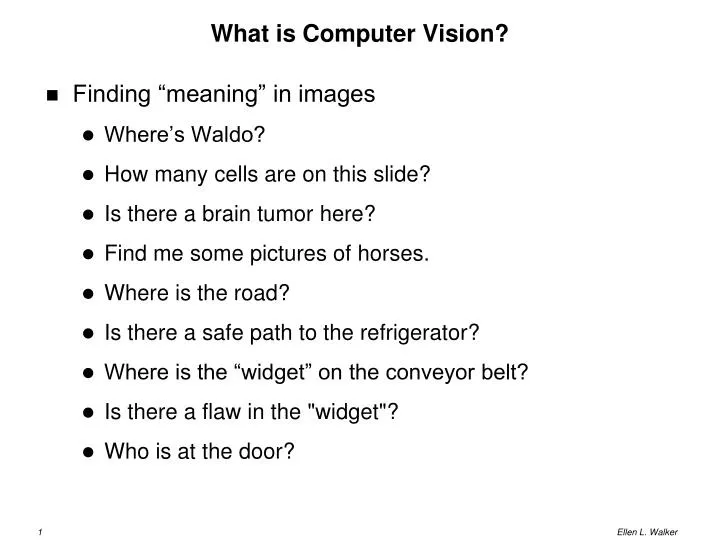
1. What is Computer Vision? • Finding “meaning” in images • Where’s Waldo? • How many cells are on this slide? • Is there a brain tumor here? • Find me some pictures of horses. • Where is the road? • Is there a safe path to the refrigerator? • Where is the “widget” on the conveyor belt? • Is there a flaw in the "widget"? • Who is at the door?

2. Some Applications of Computer Vision • Sorting envelopes with handwritten addresses (OCR) • Scanning parts for defects (machine inspection) • Highlighting suspect regions on CAT scans (medical imaging) • Creating 3D models of objects (or the earth!) based on multiple images • Alerting a driver of dangerous situations (or steering the vehicle) • Fingerprint recognition (or other biometrics) • Creating performances of CGI (computer generated imagery) characters based on real actors’ movements

3. Why is vision so difficult? • The bar is high – consider what a toddler ‘knows’ about vision • Vision is an ‘inverse problem’ . Forward: one scene => one image Reverse: one image => many possible scenes ! • The human visual system makes assumptions • Why optical illusions work (see fig. 1.3)

4. 3 Approaches to Computer Vision (Szeliski) • Scientific: derive algorithms from detailed models of the image formation process • Vision as “reverse graphics” • Statistical: use probabilistic models to describe the unknowns and noise, derive ‘most likely’ results • Engineering: Find techniques that are (relatively) simple to describe and implement, but work. • Requires careful testing to understand limitations and costs

5. Testing Vision Algorithms • Pitfall: developing an algorithm that “works” on your small set of test images used during development • Surprisingly common in early systems • Suggested 3-part strategy • Test on clean synthetic data (e.g. graphics output) • Add noise to your data and study degradation • Test on real-world data, preferably from a wide range of sources (e.g. internet data, multiple ‘standard’ datasets)

6. Engineering Approach to Vision Applications • Start with a problem to solve • Consider constraints and features of the problem • Choose candidate techniques • We will cover many techniques in class ! • If you’re doing an IRC, I’ll try to point you in the right directions to get started • Implement & evaluate one or more techniques (careful testing!) • Choose the combination of techniques that works best and finish implementation of system

7. Scientific and Statistical Approaches • Find or develop the best possible model of the physics of the system of image formation • Scene geometry, light, atmospheric effects, sensors … • Scientific: Invert the model mathematically to create recognition algorithms • Simplify as necessary to make it mathematically tractable • Take advantage of constraints / appropriate assumptions (e.g. right angles) • Statistical: Determine model (distribution) parameters and/or unknowns using Bayesian techniques • Many machine learning techniques are relevant here

8. Levels of Computer Vision • Low level (image processing) • Makes no assumptions about image content • Use similar algorithms for all images • Nearly always required as preprocessing for HL vision • Techniques from signal processing, “linear systems” • High level (image understanding) • Requires models or other knowledge about image content • Often specialized for particular types of images • Techniques from artificial intelligence (especially non-symbolic AI)

9. Overview of Topics (Szeliski, ch. 1)

10. Operations on Images • Low-level operators • Pixel operations • Neighborhood operations • Whole image operations (often neighborhood in a loop) • Multiple-image combination operations • Image subtraction (to highlight motion) • Higher-level operations • Compute features from an image (e.g. holes, perimeter) • Compute non-iconic representations

11. Object Recognition • I have a model (something I want to find) • Image (iconic) • Geometric (2D or 3D) • Pattern (image or features) • Generic model (“idea”) • I have an image (1 or more) • I have questions • Where is M in I (if at all)? • What are parameters of M that can be determined from I?

12. Top-Down vs. Bottom up • Top-down • Use knowledge to guide image processing • Example: image of “balls” - search for circles • Danger: Too much top-down reasoning leads to hallucination! • Bottom-up • Extract as much from image as possible without any models • Example: edge detection -> thresholding -> feature detection • Danger: “Correct” results might have nothing to do with the actual image contents

13. Geometry: Point Coordinates • 2D Point • x =(x, y) Actually a column vector (for matrix multiplication) • Homogeneous 2D point (includes a scale factor) • x = (x, y, w) • (2, 1, 1) = (4, 2, 2) = (6, 3, 3) = … • Transformation: • (x, y) => (x, y, 1) • (x, y, w) => (x/w, y/w) • Special case: (x, y, 0) is “point at infinity”

14. Modifying Homogeneous Points Increase y Increase x Increase w

15. Lines • L = (a, b, c) (homogeneous vector) • x*l = ax + by + c (line equation) • Normal form: L = (n_x, n_y, d) • n is the direction, d is the distance to origin • Theta = acos(n_y / n_x)

16. Transformations • 2D to 2D (3x3 matrix, multiply by homogeneous point) • Coordinates r00, r01, r10, r11 specify rotation or shearing • For rotation: r00 and r11 are cos(theta), r01 is –sin(theta) and r11 is sin(theta) • Coordinates tx and ty are translation in x and y • Coordinate s adjusts overall scale; sx and sy are 0 except for projective transform (next slide)

17. Hierarchy of 2D Transformations (Table 2.1)

18. 3D Geometry • Points: add another coordinate, (x, y, z, w) • Planes: like lines in 2D with an extra coordinate • Lines are more complicated • Possibility: represent line by 2 points on the line • Any point on the line can be represented by combination of the points • r = (lambda)p1 + (1-lambda)p2 • If 0<=lambda<=1, then r is on the segment from p1 to p2 • See 2.1 for more details and more geometric primitives!

19. 3D to 2D Transformations • These describe ways that 3D reality can be viewed on a 2D plane. • Each is a 3x4 matrix • Multiply by 3D Homogeneous vector (4 coordinates) to get a 2D homogeneous vector (3 coordinates) • Many options, see Section 2.1.4 • Most common is perspective projection

20. Perspective Projection Geometry (Simplified) See Figure 2.7

21. Simplifications of "Pinhole Model" • Image plane is between the center of projection and the object rather than behind the lens as in a camera or an eye • Objects are really imaged upside-down • All angles, etc. are the same, though • Center of projection is a virtual point (focal point of a lens) rather than a real point (pinhole) • Real lenses collect more light than pinholes • Real lenses cause some distortion (see Figure 2.13)

22. Photometric Image Formation • A surface element • (with normal N) • Reflects radiation from a single source • (with angle  to N) • Toward the sensor • (This is called irradiance) • Which senses and records it Figure 2.14

23. Light Sources • Geometry (point vs. area) • Location • Spectrum (white light, or only some wavelengths) • Environment map (measure ambient light from all directions) • Model depends on needs • Typical: sun = point at infinity • More complex model needed for soft shadows, etc.

24. Reflected Light • Diffuse reflection (Lambertian, matte) • Amount of light in a given direction (apparent brightness) depends on angle to surface normal • Specular reflection • All light reflected in one ray; angle depends on light source and surface normal Figure 2.17

25. Image Sensors • Charge couple device (CCD) • Count photons (unit of light) that hit (one counter per pixel) • (Light energy converted to electrical charge) • “Bleed” from neighboring pixels • Each pixel reports its value (scaled by resolution) • Result is a stream of numbers (0=black, MAX=white)

26. Image Sensors: CMOS • No bleed; each pixel is independently calculated • Each pixel can have an independent color filter • Common in current (2009) digital cameras Figure 2.24

27. Digital Camera Image Capture Figure 2.25

28. Color Image • Color requires 3 values to specify (3 images) • Red, green, blue (RGB) : computer monitor • Cyan, Magenta, Yellow, Black (CMYK): printing • YIQ (Y is intensity, I is “lightness”): color TV signal (Y is B/W signal) • Hue, Saturation, Intensity: Hue = pure color, saturation = density of color, intensity = b/w signal (“color-picker”) • Visible color depends on color of object, color of light, material of object, and colors of nearby objects! (There is a whole subfield of vision that “explains” color in images. See section 2.3.2 for more details and pointers)

29. Problems with Images • Geometric Distortion (e.g. barrel distortion) - from lenses • Scattering - e.g. thermal "lens" in atmosphere - fog is an extreme case • Blooming - CCD cells affect each other • Sensor cell variations - "dead cell" is an extreme case • Discretization effects (clipping or wrap around) - (256 becomes 0) • Chromatic distortion (color "spreading" effect) • Quantization effects (fitting a circle into squares, e.g.)

30. Aliasing: An Effect of Sampling • Our vision system interpolates between samples (pixels) • If not enough samples, data is ambiguous

31. Image Types • Analog image - the ideal image, with infinite precision - spatial (x,y) and intensity f(x,y) • f(x,y) is called the picture function • Digital image - sampled analog image; a discrete array I[r,c] with limited precision (rows, columns, max I) • I[r,c] is a gray-scale image • If all pixel values are 0 or 1, I[r,c] is a binary image • M[r,c] is a multispectral image. Each pixel is a vector of values, e.g. (R,G,B) • L[r,c] is a labeled image. Each pixel is a symbol denoting the outcome of a decision, e.g. grass vs. sky vs. house

32. Coordinate systems • Raster coordinate system • Derives from printing an array on a line printer • Origin (0,0) is at upper left • Row (R) increases downward; Column (C) increase to right • Cartesian coordinate system • Typical system used in mathematics • Origin (0,0) is at lower left • X increases to the right; Y increases upward • Conversions • Y = MaxRows - R ; X = C • Or, pretend X=R, Y=C then rotate your printout 90 degrees!

33. Resolution • In general, resolution is related to a sensor's measurement precision or ability to detect fine features • Nominal resolution of a sensor is the size of the scene element that images to a singel pixel on the image plane • Resolution of a camera (or an image) is also the number of rows & columns it contains (or their product), e.g. "8 megapixel resolution" • Subpixel Resolutionmeans that the precision of measurement is less than the nominal resolution (e.g. subpixel resolution of positions on a line segment)

34. Variation in Resolution

35. Quantization Errors • One pixel contains a mixture of materials • 10m x 10m area in a satellite photo • Across the edge of a painted stripe or character • Subpixel shift in location has major effect on image! • Shape distortions caused by quantization ("jaggies") • Change / loss in features • Thin stripe lost • Area varies based on resolution (e.g. circle)

36. Representing an Image • Image file header • Dimensions (#rows, #cols, #bits / pixel) • Type (binary, grayscale, color, video sequence) • Creation date • Title • History (nice) • Data • Values for all pixels, in a pre-defined order based on the format • Might be compressed (e.g. JPEG is lossy compression)

37. PNM: a simple image representation • Portable N Map • Pbm = portable bit map • Pgm = portable gray map • Ppm = portable pixel map (color image) • ImageJ reads, displays, and converts PNM images. (pbm, pgm, ppm) – and much more! • GIF, JPG and other formats can be converted (both ways) • ImageJ does not appear to convert color to grayscale • Irfanview (Windows only) reads, displays and converts

38. PNM Details • Comments can be anywhere after Px - lines begin with # • First Px (where x is an integer from 1-6) • P1/4 = binary, P2/5 = gray, P3/6 = color • P1-P3: data in ascii, P4-P6: data in binary • Next come 2 integers (#cols, #rows) • Next (unless it’s P1 or P4) comes 1 integer (#greylevels) • The rest of the image is pixel values from 0 to #greylevels – 1 (If color: red image, then green, then blue)

39. PGM image example • This one is really boring! P2 3 2 4 0 0 0 1 2 3

40. Other Image Formats • GIF (Compuserve - commercial) • 8-bit color (uses a colormap) • LZW lossless compression available • TIFF (Aldus Corp., for scanners) • Multiple images, 1-24 bits / pixel color • Lossy or lossless compression available • JPEG (Joint Photographic Experts Group - free) • Lossy compression • Real-time encoding/decoding in hardware • Up to 64K x 64K x 24bits

41. Specifying a vision system • Inputs • Sensor(s) OR someone else's images • Environment (e.g. light(s), fixtures for holding objects, etc.) OR unconstrained environments • Resolution & formats of image(s) • Algorithms • To be studied in detail later(!) • Results • Image(s) • Non-iconic results

42. If you're doing an IRC… (Example from 2002) • What is the goal of your project? • Eye-tracking to control a cursor - hands-free game operation • How will you get data (see "Inputs" last slide) • Camera above monitor; user at (relatively) fixed distance • Determine what kind of results you need • Outputs to control cursor • How will you judge success? • User is satisfied that cursor does what he/she wants • Works for many users, under range of conditions

43. Staging your project • What can be done in 3 weeks? 6 weeks? 9 weeks? • Find the eyes in a single image [DONE] • Reliably track eye direction between a single pair of images (output "left", "right", "up", "down") [DONE] • Use a continuous input stream (preferably real time) [NOT DONE] • Program defensively • Back up early and often! (and in many places) • Keep printouts as last-ditch backups • When a milestone is reached, make a copy of the code and freeze it! (These can be smaller than the 3-week ideas above) • When time runs out, submit and present your best frozen milestone.