Download
1 / 60
600 likes | 658 Views
Q 2-31. B = - 1/3A + 2 B = - A + 4. Min 3A + 4B s.t. 1A + 3B ≧ 6 1A + 1B ≧ 4 A, B ≧ 0. B. B = - A + 4. Feasible Region. Objective Function = 3A + 4B Optimal Solution A = 3, B = 1. Objective Function Value = 3(3) + 4(1) = 13. B = - 1/3A + 2. A. Q 2-38 a. Let

E N D
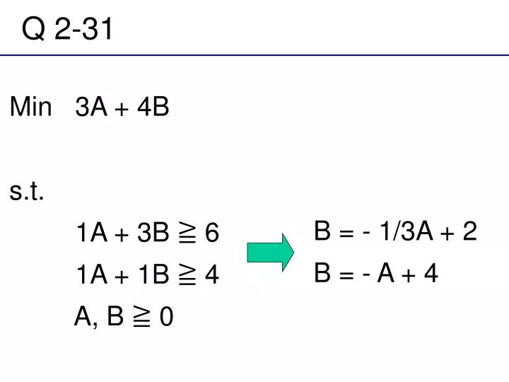
Q 2-31 B = - 1/3A +2 B =- A + 4 Min 3A + 4B s.t. 1A + 3B ≧ 6 1A + 1B ≧ 4 A, B ≧ 0
B B =- A + 4 Feasible Region Objective Function = 3A + 4B Optimal SolutionA = 3, B = 1 Objective Function Value = 3(3) + 4(1) = 13 B = - 1/3A +2 A
Q 2-38 a. Let S = yards of the standard grade material / frame P = yards of the professional grade material / frame Min 7.50S + 9.00P s.t. 0.10S + 0.30P ≧ 6 carbon fiber (at least 20% of 30 yards) 0.06S + 0.12P ≦ 3 kevlar (no more than 10% of 30 yards) S + P = 30 total S, P ≧ 0
P Total Extreme Point S = 10, P = 20 Feasible region is the line segment Kevlar Carbon fiber Extreme Point S = 15, P = 15 S
Q 2-38 c. 255.00 > 247.50 Therefore, the optimal solution is S = 15, P = 15
Q 2-38 d. Changing is only this value (From 9.00 to 8.00) Min 7.50S + 8.00P s.t. 0.10S + 0.30P ≧ 6 carbon fiber (at least 20% of 30 yards) 0.06S + 0.12P ≦ 3 kevlar (no more than 10% of 30 yards) S + P = 30 total S, P ≧ 0 Therefore, optimal solution does not change: S = 15, and P =15 New optimal solution value = 7.50(15) + 8(15) = $232.50
Q 2-38 e. At $7.40 per yard, the optimal solution is S = 10, P = 20. So, the optimal solution is changed. The value of the optimal solution is reduced to 7.50 (10) + 7.40 (20) = 223.00. A lower price for the professional grade will change the optimal solution.
Q 3-7 a. From figure 3.14, Optimal solution: U = 800, H = 1200 Estimated Annual Return 3(800) + 5(1200) = $8400
Q 3-7 b. Constraints 1 and 2 because of 0 at Slack/Surplus column. All funds available are being fully utilized and the maximum risk is being incurred.
Q 3-7 c. A unit increase in the RHS of Funds Avail makes 0.09 improvement in the value of the objective function. Risk Max also makes 1.33 improvement in the value of the objective function. A unit increase in the RHS of U.S. Oil Max makes no improvement in the objective function value.
Q 3-7 d. NO A unit increase in the RHS of U.S. Oil Max makes no improvement in the objective function value.
Q 3-10 a. From figure 3.16, Optimal solution: S = 4,000, M = 10,000 Estimated total risk = 8(4,000) + 3(10,000) = 62,000
Q 3-10 c, d, e, f (c) 5(4,000) + 4(10,000) = $60,000 (d) 60,000/1,200,000 = 0.05 (e) 0.057 (f) 0.057(100) = 5.7
A two-variable linear programming problem Max s.t. and For any LP problem with n decision variables, each CPF (Corner Point Feasible) solution lies at the intersection of n constraint boundaries; i.e., the simultaneous solution of a system of n constraint boundary equations.
Max s.t.
Original Form Augmented Form Max s.t. Max s.t. (1) Matrix Form (2)
Matrix Form (2) is Max s.t. (3) or Max s.t. (4) where
Then, we have Max s.t. (5) (6) where
Eq. (6) becomes (7) Putting Eq. (7) into (5), we have (8) So, (9) (10)
Eq. (10) can be expressed by (11) From Eq. (2), (12)
The Overall Procedure 1.Initialization: Same as for the original simplex method. 2.Iteration: Step 1 Determine the entering basic variable: Same as for the Simplex method.
Step 2 Determine the leaving basic variable: Same as for the original simplex method, except calculate only the numbers required to do this [the coefficients of the entering basic variable in every equation but Eq. (0), and then, for each strictly positive coefficient, the right-hand side of that equation].
Step 3 Determine the new BF solution: Derive and set 3.Optimality test: Same as for the original simplex method, except calculate only the numbers required to do this test, i.e., the coefficients of the nonbasic variables in Eq. (0).
Fundamental Insight Z RHS Z 1 Row0 0 Row1~N
Coefficient of: Right Side Iteration BV -3 -5 0 0 0 0 1 0 1 0 0 4 0 0 2 0 1 0 12 3 2 0 0 1 18
Coefficient of: Right Side Iteration BV 0 0 0 1 0 1 0 0 4 1 0 1 0 0 6 3 0 0 -1 1 6
Coefficient of: Right Side Iteration BV -3 0 0 0 1 0 1 0 0 4 1 0 1 0 0 6 3 0 0 -1 1 6
Coefficient of: Right Side Iteration BV -3 0 0 0 1 0 1 0 0 4 1 0 1 0 0 6 3 0 0 -1 1 6
so Coefficient of: Right Side Iteration BV -3 0 0 0 30 1 0 1 0 0 4 1 0 1 0 0 6 3 0 0 -1 1 6
4 6 minimum The most negative coefficient Coefficient of: Right Side Iteration BV -3 0 0 0 30 1 0 1 0 0 4 1 0 1 0 0 6 3 0 0 -1 1 6
Coefficient of: Right Side Iteration BV 0 0 0 0 0 1 2 2 0 1 0 0 6 1 0 0 2
Coefficient of: Right Side Iteration BV 0 0 0 1 0 0 1 2 2 0 1 0 0 6 1 0 0 2
so Coefficient of: Right Side Iteration BV 0 0 0 1 36 0 0 1 2 2 0 1 0 0 6 1 0 0 2
One of the most important discoveries in the early development of linear programming was the concept of duality. Every linear programming problem is associated with another linear programming problem called the dual. The relationships between the dual problem and the original problem (called the primal) prove to be extremely useful in a variety of ways.
Primal and Dual Problems Primal Problem Dual Problem Max s.t. Min s.t. for for for for The dual problem uses exactly the same parameters as the primal problem, but in different location.
In matrix notation Primal Problem Dual Problem Maximize subject to Minimize subject to Where and are row vectors but and are column vectors.
Example Dual Problem Primal Problem Min s.t. Max s.t.
Primal Problem in Matrix Form Dual Problem in Matrix Form Max s.t. Min s.t.
Primal-dual table for linear programming Primal Problem Coefficient of: Right Side Coefficient of: Coefficients for Objective Function (Minimize) Dual Problem VI VI VI Right Side Coefficients for Objective Function (Maximize)
Relationships between Primal and Dual Problems One Problem Other Problem Constraint Variable Objective function Right sides Minimization Maximization Variables Constraints Unrestricted Constraints Variables Unrestricted
The feasible solutions for a dual problem are those that satisfy the condition of optimality for its primal problem. A maximum value of Z in a primal problem equals the minimum value of W in the dual problem.
Rationale: Primal to Dual Reformulation Lagrangian Function Max cx s.t. Ax b x 0 L(X,Y) = cx - y(Ax - b) = yb + (c - yA) x = c-yA Min yb s.t. yA c y 0
The following relation is always maintained yAx yb (from Primal: Ax b) yAx cx (from Dual : yA c) From (1) and (2), we have cx yAx yb At optimality cx* = y*Ax* = y*b is always maintained. (1) (2) (3) (4)
“Complementary slackness Conditions” are obtained from (4) ( c - y*A ) x* = 0 y*( b - Ax* ) = 0 xj* > 0 y*aj = cj , y*aj> cjxj* = 0 yi* > 0 aix* = bi , ai x*<biyi* = 0 (5) (6)
Any pair of primal and dual problems can be converted to each other. The dual of a dual problem always is the primal problem.