Download
1 / 26
260 likes | 418 Views
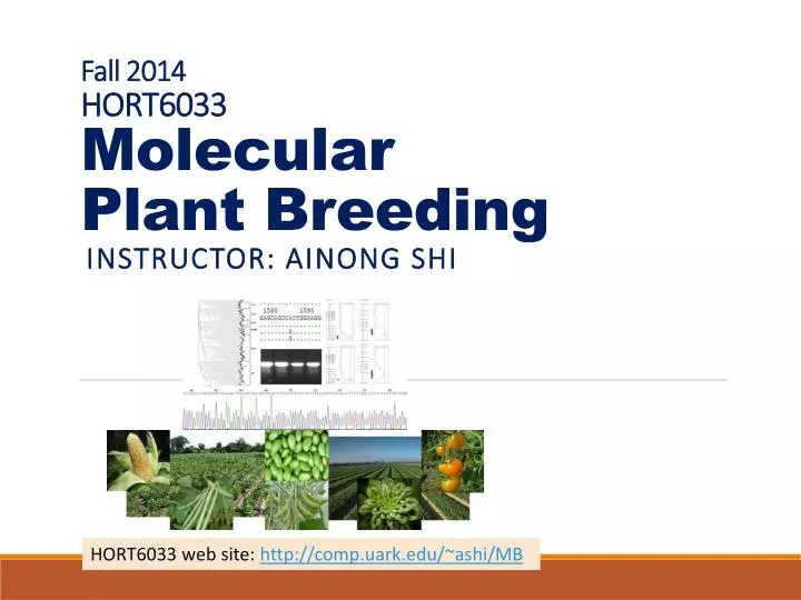
Fall 2014 HORT6033 Molecular Plant B reeding. Instructor: Ainong Shi. HORT6033 web site: http://comp.uark.edu/~ashi/MB. Fall 2014 HORT6033 Molecular Plant Breeding Lecture 9 (09/22/2014). Genetic map construction Genetic mapping Example Homework Reading.

E N D
Fall 2014HORT6033Molecular Plant Breeding Instructor: Ainong Shi HORT6033 web site: http://comp.uark.edu/~ashi/MB
Fall 2014 HORT6033 Molecular Plant Breeding Lecture 9 (09/22/2014) • Genetic map construction • Genetic mapping • Example • Homework • Reading
In classic genetics, genes can be mapped to specific locations on chromosomes. Genetic map: A graphic representation of the arrangement of genes or DNA sequences on a chromosome. Also called gene map. Locating and identifying genes in a genetic map is called genetic mapping.
A linkage map describes the linear order of markers (such as SSRs and SNPs) within a linkage group. A linkage map = a genetic map. Genetic mapping (linkage mapping) means to build genetic map(s) with a set of markers (such as SSRs and/or SNPs). It can map only one genetic map or whole genome maps of a species. Usually, what we say ‘conduct linkage mapping’ means we map a major gene of a trait to a genetic map (linkage group (LG) or chromosome). What we say ‘conduct QTL mapping’ means we map a QTL (quantitative loci trait) to one LG (chromosome) or several LGs (chromosomes) M1 M1 M1 0.1cM 0.1cM 0.1cM M2 M2 M2 0.2cM 0.2cM 0.2cM M3 M3 M3 0.1cM 0.25cM T1 (flower color) 0.25cM 0.15cM M4 M4 M4 0.1cM 0.1cM 0.1cM M6 M5 M6 Linkage map LG QTL mapping
Cowpea Whole Genome Genetic Maps 11 chromosome 928 EST-SNPs Fig. S1. Graphical representation of the consensus cowpea genetic linkage map constructed by using 928 EST-derived SNP markers segregating in six recombinant inbred populations. Muchero et al. 2009. PNAS 106:18159–18164.
Cowpea Bacterial Blight CoBB susceptible CoBB resistance
QTL mapping for CoBB Resistance • Three QTLs, CoBB1, CoBB2, and CoBB3, were reported to be linked to CoBB resistance on linkage group LG3, LG5 and LG9 of cowpea (Agbicodo et al. 2010). • Two SNP markers, CP08_5433936 and CP02_50192757 were identified to be associated with CoBB resistance located at the same regions of CoBB1 and CoBB2, respectively. The accuracy of selecting resistance lines was 86.7% based on the data of 201 cowpea lines from this study. CP02_50192757 CP08_5433936 Agbicodoet al. 2010. Euphytica 175:215-225
Estimate the linkage of two alleles in a segregating population • Recombination fraction • LOD score • Haldane and Kosambi mapping function
Recombination Frequency • Recombination fraction is a measure of the distance between two loci. • Two loci that show 1% recombination are defined as being 1 centimorgan (cM) apart on a genetic map. • 1 map unit = 1 cM (centimorgan) • Two genes that undergo independent assortment have recombination frequency of 50 percent and are located on nonhomologous chromosomes or far apart on the same chromosome = unlinked • Genes with recombination frequencies less than 50 percent are on the same chromosome = linked
Calculation of Recombination Frequency • The percentage of recombinant progeny produced in a cross is called the recombination frequency, which is calculated as follows:
LOD SCORE • The LOD score is calculated as follows: • LOD = Z = Log10 probability of birth sequence with a given linkage probability of birth sequence with no linkage • By convention, a LOD score greater than 3.0 is considered evidence for linkage. • On the other hand, a LOD score less than -2.0 is considered evidence to exclude linkage.
LOD Score Analysis • The likelihood ratio as defined by :- L(pedigree| = x) L(pedigree | = 0.50) • where represents the recombination fraction and where 0 x 0.49. • L.R. = • TheLOD score (z) is the log10 (L.R.)
Method to evaluate the statistical significance Maximum-likelihood analysis, which estimates the “most likely” value of the recombination fraction Ø as well as the odds in favour of linkage versus nonlinkage. • Given by Conditional probability L(data 1 Ø), which is the likelihood of obtaining the data if the genesare linked and have a recombination fraction of Ø. Likelihood of obtaining one recombinant and seven nonrecombinants when the recombination fraction is Ø is proportional to Ø1(1–Ø)7, Where:Ø is, by definition, the probability of obtaining a recombinant , (I – Ø) is the probability of obtaining a nonrecombinant.
Mappingfunction • The genetic distance between locus A and locus B is defined as the average number of crossovers occurring in the interval AB. • Mapping function is use to translate recombination fractions into genetic distances. • In 1919 the British geneticist J, B. S. Haldane proposed such Mapping function • Haldane defined the genetic distance, x, between two loci as the average number of crossovers per meiosis in the interval between the two loci.
What is Haldane ’s mapping function ? • Assumptions: crossovers occurred at random along the chromosome and that the probability of a crossover at one position along the chromosome was independent of the probability of a crossover at another position. • Using these assumptions, he derived the following relationship between • Ø, the recombination fraction and • x ,the genetic distance (in morgans): Ø=1/2(1-e-2x) or equivalently, X=-1/2ln(1-2Ø)
Genetic distance between two loci increases, the recombination fraction approaches a limiting value of 0.5. • Cytological observations of meiosis indicate that the average number of crossovers undergone by the chromosome pairs of a germ-line cell during meiosis is 33. • Therefore, the average genetic length of a human chromosome is about 1.4 morgans, or about140 centimorgans.
Suppose: A SNP marker M1 [A/C] is linked to the pea color gene ‘T1’ with the recombination rate r. In the BC1F1(P2) population, the genotypes and phenotypes and their count are below. M1 0.064 cM T1 Haldane ’s mapping function X=-1/2ln(1-2Ø) = -0.5*ln(1-2*0.06) =0.064cM M1 0.06 cM T1 Kosambi function using the formula CM1T1= 1/4ln [(1+2r)/(1-2r)] = 0.25 * ln[(1+2*0.06)/(1-2*0.06)] = 0.06 cM
Construction of Genetic Map using JoinMap • Download and install JoinMap 4.1 at http://www.kyazma.nl/index.php/mc.JoinMap/sc.Evaluate/ • Please also download the manual at http://www.kyazma.nl/index.php/mc.JoinMap/sc.Manual/ • The JionMap slideshow at http://www.kyazma.nl/docs/JM4slideshow.pdf • Example data at http://comp.uark.edu/~ashi/MB/lecture/geneticMapExample1.loc • http://comp.uark.edu/~ashi/MB/lecture/geneticMap_rowDataExmaple.xlsb ;create genetic maps name=GeneticMapExample1 popt=F2 ; population generation nloc=720 ; number of markers nind=184 ; population size M042843 HHHHHHHBHBHBAAHHBAHHHBBHHHHHHBHABHAHBBHHAABHHABBAAHBHHHAHHBHHHBHBBHBHABAHHHHHHHBABBAHHHHBBAHHBBAHHHBHHXABBAHHBBBHHAHBAXBABHAHHHABAHHHAABHBAHHBAHBBHAAHAAHBHABBAAHHBHAHHABBBAAAHBHHBBBHBH ………………………………………………. M050787 HHHBHAHHAHBHAHBHAAHHHHHAABHHBHABHHBHBHHBAHAHHBHAHBHBBBBHAHHBHHBBHHAHHAHHBHHHHBAAHAHHBHBHABHBHHBXHHHHBBHHBHHHBHHAHHHHAAXAHBHHHBHHHHBHBBBHHAHBHABAHBBHABABHHHBHHHHBHHHHAABHAHBBBAAHBHBHHAH
Linkage mapping of wheat powdery mildew resistance(wheat-pm.pps) Example
Homework • 1. Create 6 genetic maps of spinach using Zebu F2 SNP data • 1a. Using a JoinMapformat file: spinach_ZebuF2_a.loc • 1b. Using SNP data: Zebu_F2_SNP.xlsb • 1c. Using GBS sequence data. • Request: 1a • 1b and 1c are extra work for bonus.
Reading • Muchero, M., N.N. Diop, P.R. Bhat, R.D. Fenton, S. Wanamaker, M. Pottorff, S. Hearne, N. Cisse, C. Fatokun, J. D. Ehlers, P.A. Roberts, and T.J. Close. 2009. A consensus genetic map of cowpea [Vignaunguiculata (L.) Walp.] and synteny based on EST-derived SNPs. PNAS 106:18159–18164 (http://www.pnas.org/content/106/43/18159.full.pdf) • Agbicodo, E.M., C.A. Fatokun, R. Bandyopadhyay, K. Wydra, N.N. Diop, W. Mucher, J.D. Ehlers, P.A. Roberts, T.J. Close, R.G.F. Visser, and C.G. van der Linden. 2010. Identification of markers associated with bacterial blight resistance loci in cowpea. Euphytica 175:215-226(http://link.springer.com/article/10.1007/s10681-010-0164-5/fulltext.html) • Genetic Mapping: http://web.pdx.edu/~justc/courses/IntroGenetics/Ch4&5GeneLinkageRecombinationAnalysis.ppt • agrico.rakesh_linkage • Genetic_mapping-100917050507-phpapp01