Variational principle

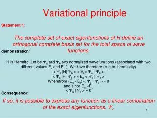
1. Statement 1: The complete set of exact eigenfunctions of H define an orthogonal complete basis set for the total space of wave functions.H is Hermitic. Let be Ya and Yb two normalized wavefunctions (associated with two different values Ea and Eb ). We have therefore (due to hermiticity) < Ya |H| Yb > = Ea< Ya | Yb > < Ya |H| Yb > = Eb < Ya | Yb > Wherefrom (Ea - Eb) < Ya | Yb > = 0 and since EaEb < Ya | Yb > = 0 If so, it is possible to express any function as a linear combination of the exact eigenfunctions, Yi. Variational principle demonstration: Consequence:

2. Statement 2: Variational principle The energy associated with Y a function is always above that of the eigenfunction of lowest energy: E0.Y is not a eigenfunction; it is associated with an energy <E> that is an average energy (mean value) A mean value is always intermediate relative to extreme: Greater than the smallest! <E> > E0

3. Mean value • If Y1 and Y2 are associated with the same eigenvalue o: O(aY1 +bY2)=o(aY1 +bY2) • If not O(aY1 +bY2)=o1(aY1 )+o2(bY2) we define <O> = (a2o1+b2o2)/(a2+b2) Dirac notations

4. Statement 2: The energy associated with Y a function is always above that of the eigenfunction of lowest energy: E0.Ya and Yb are two eigenfunctions< Ya |H| = < Ya | Ea and |H| Yb > = Eb | Yb> wherefrom < Ya |H| Yb > = Eadab From statement 1, Y is a linear combination of Ya s | Ya >= Saca| Ya > let multiply the left by < Ya |; this leads to only one term ca= < Ya |Y > and similarly c*a= < Y |Ya > then | Y >= Sa< Ya |Y > | Ya > Variational principle

5. Statement 2, normalization: Ya and Yb are two eigenfunctionsassociated to Ea and Eb From statement 1, Y is a linear combination of Ya s | Y >= Saca| Ya > then < Y | Y > =Sa,bca< Ya |Yb> cb < Y | Y > = Sa,ca2< Ya |Ya> = Sa,ca2= 1 Variational principle

6. Statement 2, Demonstration: Variational principle < Y |H | Y > = Sa,bca < Ya |H | Yb > cb < Y |H | Y > = Sa,bEa < Ya | Yb > cb < Y |H | Y > = Sa,bEa cadab cb < Y |H | Y > = Sa,Ea ca2 >Sa,E0 ca2 = E0 E > E0 An non-exact solution has always a higher energy than the lowest exact solution

7. Using Dirac notation Ya and Yb are two eigenfunctions< Ya |H| = < Ya | Ea and |H| Yb > = Eb | Yb > wherefrom < Ya |H| Yb > = Eada From statement 1, Y is a linear combination of Ya s | Ya >= Saca| Ya > Let multiplie the left by < Ya |; this leads to only one term ca= < Ya |Y > and similarly c*a= < Y |Ya > then < Y | Y > = Sa,bca< Ya |Yb> cb < Y | Y > = Sa,b< Ya |Y > < Ya |Yb> < Yb|Y > = Sa,b< Ya |Y > dab < Yb|Y > < Y | Y > = Sa,|< Ya |Y >|2 =1 Demonstration < Y |H | Y > = Sa,b< Y | Ya > < Ya |H | Yb > < Y b|Y > < Y |H | Y > = Sa,bEa < Y | Ya > < Ya | Yb > < Y b|Y > < Y |H | Y > = Sa,bEa < Y | Ya > dab < Y b|Y > < Y |H | Y > = Sa,Ea |< Ya |Y >|2 >Sa,E0|< Ya |Y >|2 = E0 < Y |H | Y > >E0

8. Variation principle Given an approximate expression that depends on parameters, we must determine the parameters to minimize the energy. Within LCAO, an MO is a linear combination of AOs: We have then to chose the coefficients so to minimize the energy. Note that the variational principle is not restricted to cases of linear combinations.

9. A mean value is always higher than the lowest value ! c32 c22 c12 c02

10. Slater exponent for He F = where Z* is a parameter <E> = - Z*2/2 u.a. <T> = + Z*2/2 u.a. <V> = <F(1,Z*)|-Z*/r|F(1,Z*)> using <F(1,Z*)|1/r|F(1,Z*)> = Z* u.a. <V> = -Z*<F(1,Z*)|1/r|F(1,Z*)> = -Z*2u.a. Next slide

11. <F(1,Z*)|1/r|F(1,Z*)> = Z* u.a. demonstration

12. Slater exponent for He F = where Z* is a parameter

13. Slater exponent for He F = where Z* is a parameter Search for the energy minimum

14. LCAO Y is a linear combination of N fa s | Y >= Saca| fa > Atomic orbitals Worse description than Y an approximate function Using parameters: ca There are N coeffcients to determine Let minimize E with respect to each of them Therefore, there is a set of N equations, dE/dc = 0 This seems fine; however there is a problem; Which is the problem?

15. Lagrangian There is a constraint due to normalization: the N coefficients are not independent. We search the minimum of a function L of N+1 variables Which “makes no difference with H” L = <Y| Y > - E [<Y| Y > - 1 ] There is a set of linear expressions to derive dL/dc = 0 Should be 0 Joseph Louis de Lagrange French 1736 - 1831

16. Secular determinant Solving | Hij-ESij| =0, we find the Eis. This is a N degree equation of E to be solved. From N AOs, we find N energies and N MOs. We find simultaneously E and Y (eigenfunction and eigenvalues).

17. LCAO Assuming no changein the AOs *, the MOs correspond to a unitary change of the basis set of AOs. MOs are orthogonal and normalized. Neglecting overlaps, Src2ir=1 for a MO, Yi and Sic2ir=1 for a AO, fi ; the AOs are distributed among the MOs * This is not the case for self consistent methods. Sum over r atoms for a given iorbital Sum over iorbitals for a given r atom

18. Schrödinger equation for LCAO HY = EY H SiciFi = ESiciFi Let multiply on the left by Fj, integrate and develop Sici<|H |Fi > = ESici <Fj |Fi> Sici (Hij-E Sij ) = 0 This is the set of linear equation solved for | Hij-ES ij |= 0 secular determinant Erwin Rudolf Josef Alexander Schrödinger Austrian 1887 –1961 The complete set of MOs are solution (not only the lowest). Our first approach from the variational principle emphasized the solution of lowest energy Every extreme (derivative=0) is a physical solution!

19. Hückel Theory In the 1930's a theory was devised by Hückel to treat the p electrons of conjugated systems such as aromatic hydrocarbon systems, benzene and naphthalene. Only p electron MO's are included because these determine the general properties of these molecules and the s electrons are ignored. This is referred to as sigma-pi separability. The extended Hückel Theory introduced by Lipscomb and Hoffmann (1962) applies to all the electrons. Erich Armand Arthur Joseph Hückel German 1896-1980 Never awarded the Nobel prize! Also known for Debye-Hückel theory of electrolytic solutions

20. Hückel Theory We consider only 2pZ orbitals Two parameters: The atomic 2p energy level: E(2pZ) = a (~ -11.4 eV) The resonance integral for adjacent 2p orbitals Hij(C=C) = b (~ -3 eV) E = a + x b  -x= (a – E)/ b We chose defining b as negative Sij = dij (the overlap is neglected). Erich Armand Arthur Joseph Hückel German 1896-1980 Never awarded the Nobel prize! Also known for Debye-Hückel theory of electrolytic solutions

21. SLATER KOSTER Slater Koster for metal atoms : 9 orbitals s, p et d Several overlaps ss, sps, sds, pps, ppp, pds, pdp, dds, ddp, ddd. Phys. Rev B 94 (1954) 1498

22. EHT Theory • Only valence orbitals are described • AOs are Slater orbitals • Parameters are the Hii (atomic energy levels) • The Slater exponents • The Overlap, Sij, are rigorously calculated from the geometry and the AOs • The resonance integrals, Hij, are derived from the Sij. Wolfsberg-Helmoltz formula Hij = 1.75 (Hii+Hjj)/2 Sij

23. For linear and cyclic systems (with n atoms), general solutions exist. • Linear: • Cyclic: • For linear polyenes the energy gap is given as: Polyenes Charles Alfred Coulson (1910-1974), English

24. Extension to heteroatoms

25. | Hij-ESij|= 0 1 means that the atoms 2 and 4 are connected, The determinant is symmetric relative to the diagonal

26. | Hij-ESij|= 0 This is an N degree equation of x

27. | Ei-x|= 0solving is a diagonalization problem A set of first degree equations: E=Ei associated with Yi

28. The diagonalization is a unitary transformation OMs are orthogonal thus Srcricrj= dij If i=j, the sum of the coefficient’s squares for a given atom is 1 (normalization) If i≠j, the sum of the products of coefficients is 0 (orthogonality) The matrix of coefficients is unitary wherefrom = Sicricsj= dij If i=j, the sum of the coefficient’s squares for a given orbital is 1 AOs are distributed among all the MOs If i≠j, the sum of the products of coefficients is 0 If all the orbitals were filled, there would be no interaction: all the r-s bond indices should be zero.

29. C2H42 e in 2 orbitals as in H2We have solved the problem using symmetryand without solving the secular equation. Inputs are what is in the secular determinant : a b and connectivity Outputs are orbitals, energies, total energies, charges and bond indices

30. C2H4without overlap N-1 linear equations; the last one is redundant.

31. C2H4including overlap 4e repulsion E2 = (b -ES)2 E = ±(b -ES) Mulliken Overlap populations

32. 2 OA interaction modifying a -b2/ D • (D/2 -E) (-D/2 -E) = b2 E2-(D2/4) = b2 • E2 = b2 +(D2/4) • E = ±√[b2 +(D2/4)] • If D = 0, E+ = b • If b <<D, • E+ = (D/2) (1+4b2/ D2) 0.5 • E+ = (D/2) (1+2b2/ D2) = D/2 (1 +2b2/ D) • E+ - E = b2/ D «2nd order Perturbation term -D/2 D/2 b2/ D The geometric mean of b and D/2

33. Butadiene The topology is C1 bond C2, C2 bond to C3 and C3 bond to C4 A linear model contains the information with more symmetry (the topology does not distinguish between cis and trans)

34. Conservation of Orbital Symmetry H C Longuet-Higgins E W Abrahamson The Molecular orbitals are solution of the symmetry operators of the molecule. MOs from different symmetry groups do not mix. Hugh ChristopherLonguet-Higgins 1923-2004

35. S or A Butadieneusing symmetry for the topology S 0 0 A

36. S ButadieneSymmetric Mind that symmetry 1 is for all the atoms Not the reduced part = 0 x2 - x - 1 = 0 x = (1 ± √5)/2 Golden numbers 1.618 and -0.618 Coefficients - (1 ± √5)/2 c1 + c2 = 0 and normalization c12 + c22 = ½ c = 0.3717 and 0.6015 -0.618 1.618

37. Golden ratio  Golden ratio conjugateF

38. Golden ratio Golden ratio conjugate a= √(b2+(2b)2) =b(1+√5) a= b(1+√5) b 2b

39. Polyclete and Durer

40. x2 = 1+x The medial right triangle of this "golden" pyramid (see diagram), with sides              is interesting in its own right, demonstrating via the Pythagorean theorem the relationship or

41. Fibonacci recursion,irrational numbers (incommensurable) Rabbit population, assuming that: In the "zeroth" month, there is one pair of rabbit In the first month, the first pair begets another pair In the second month, both pairs of rabbits have another pair, and the first pair dies. In the third month, the second pair and the new two pairs have a total of three new pairs, and the older second pair.

42. Spirale constructions,in nature,in music..Related ?The Doctrine of the Mean (中庸, py Zhōngyōng) is one of the Four Books, part of the Confucian canonical scriptures.

43. Pentagon, icosahedra  =1.618 F=1/ =0.618 2

44. S ButadieneSymmetric Recipe to build the same determinant Express along the AOs and gather interactions with equivalent atoms Mind that symmetry reduction makes the normalization incomplete.

45. A ButadieneAntisymmetric Mind that symmetry 1 is for all the atoms Not the reduced part x2 + x - 1 = 0 x = - (1 ± √5)/2 Golden numbers 0.618 and -1.618 Coefficients (1 ± √5)/2 c1 + c2 = 0 and normalization c12 + c22 = ½ c = 0.3717 and 0.6015 0.618 -1.618

46. A ButadieneAntisymmetric Recipe to build the same determinant Express along the AOs and gather interactions with equivalent atoms Mind that symmetry reduction makes the normalization incomplete.

47. Butadiene Small 0.3717 Large 0.6015 Large 0.6015 Small 0.3717 Large 0.6015 Small 0.3717 The number of nodes increases, the amplitude is large at the middle for the extreme; it is large on the edges for the Frontier orbitals.

48. Butadiene -.3717 -.6015 -1.618 0.3717 0.6015 0.6015 -.3717 -.618 0.6015 -.3717 -.6015 0.3717 0.618 -.3717 0.6015 0.6015 1.618 0.6015 0.3717

49. Butadiene Bonding orders Ground state 0.894 0.894 0.447 No initial statement that distinguishes 1-2 from 2-3

50. Butadiene C=C – C=C Bonding orders Ground state 1.35Ả 1.35Ả 1.46Ả No initial statement that distinguishes 1-2 from 2-3 Matches the Lewis formula and indicates the stabilization due to delocalization