Download
1 / 71
810 likes | 1.32k Views
Marine Biogeochemical and Ecosystem Modeling. Michael Schulz MARUM -- Center for Marine Environmental Sciences and Faculty of Geosciences, University of Bremen. 9:15 - 9:45 1. Introduction (Lecture) - The global carbon cycle, CO 2 in seawater - “Biological pumps”

E N D
Marine Biogeochemical and Ecosystem Modeling Michael Schulz MARUM -- Center for Marine Environmental Sciences and Faculty of Geosciences, University of Bremen
9:15 - 9:45 1. Introduction (Lecture)- The global carbon cycle, CO2 in seawater - “Biological pumps” - Reservoir or box models 2.Modeling Marine Nutrient and Carbon Cycles (Box-Model Exercise)- Global oceanic phosphate distribution - Nutrient – productivity interactions - Oceanic carbon budget and large-scale ocean circulation 10:45 - 11:00 break
11:00 – 12:30 2. cont'd- Circulation-productivity feedback in the global ocean 3. State-of-the-art Biogeochemical Models (Lecture)- 2D and 3D Models- Included tracers and processes 4. Marine Ecosystem Models (Lecture) - Why ecosystem models? - Ecosystem models in paleoceanography
Course Material www.geo.uni-bremen.de/geomod/ staff/mschulz/lehre/ECOLMAS_Modeling/ This presentation Box-model exercises
Basic Literature Najjar, R. G., Marine biogeochemistry. in Climate system modeling, edited by Trenberth, K. E., pp. 241-280, Cambridge University Press, Cambridge, 1992. Rodhe, H., Modeling biogeochemical cycles. in Global biogeochemical cycles, edited by Butcher, S. S., R. J. Charlson, G. H. Orians and G. V. Wolfe, pp. 55-72, Academic Press, London, 1992. Sarmiento, J. L., and N. Gruber, Ocean biogeochemical dynamics, pp. 503, Princeton University Press, Princeton, 2006. Walker, J. C. G., Numerical adventures with geochemical cycles, 192 pp., Oxford University Press, New York, 1991.
For a climatologist biogeochemical cycles usually translates into carbon cycle. Ruddiman (2001)
Carbon-Cycle – Characteristic Timescales Reservoir Sizes in [Gt C] Fluxes in [Gt C / yr] Sundquist (1993, Science)
Average surface- Water composition CO2 0.5 % HCO3- 89.0 % CO32- 10.5 % Thurman & Trujillo (2002)
Biological Productivity in the Ocean Nutrients: P, N, (Si, Fe) Ruddiman (2001)
The Biological Pump Atmosphere CO 2 CO 2 Primary Production Inorgan. C Organ. C ® Particle-Flux Ocean Remineralisation Organ. C CO ® 2 Sediments Fig. courtesy of A. Körtzinger
Photic Zone Aphotic Zone Sediments
Biogenic Calcium Carbonate Production Raises Dissolved CO2 Concentration pH Reaction: (1) Biogenic carbonate uptake (2) More bicarbonate dissociates (3) More CO2 is formed
The Calcium Carbonate Pump Atmosphere CO 2 CO 2 Biogenic CaCO3 Formation 3 Lysocline Ocean CaCO3 Dissolution CO 2- 3 Fig. courtesy of A. Körtzinger
Reservoir or Box Models • Reservoir = an amount of material defined by certain physical, chemical or biological characteristics that, under the particular consideration, can be regarded as homogeneous. (Examples: CO2 in the atmosphere, Carbon in living organic matter in the oceanic surface layer) • Flux = the amount of material transferred from one reservoir to another per unit time
Single Reservoir Case Reservoir (mass M) Flux In Flux Out
Basic Math of Box Models (Rate of change of mass in reservoir) = (Flux in) – (Flux out) + Sources – Sinks Or, for concentration (C [mol/m3]) and water flux (Q [m3/s]):
Numerical Solution of Box-Model Equations Solution by finite-difference method (approximation!) “Euler Method” Initial Condition Time (in steps of Dt)
Numerical Solution of Box-Model Equations Solution by finite-difference method (approximation!) Initial Condition
Numerical Solution of Box-Model Equations Solution by finite-difference method (approximation!) “Euler Method” Initial Condition Time (in steps of Dt)
Euler Method M M(tn+1) “Prediction” Slope = Fi(tn) - Fo(tn) + SMS(tn) Error True Value M(tn) Dt tn tn+1 t Assumption: Slope at time tn remains constant throughout time interval Dt
Coupled Reservoirs F12 Reservoir 2 (mass M2) Reservoir 1 (mass M1) F21 Principle of mass-conservation requiresM1 + M2 = const.
Large-Scale Ocean Circulation (after Broecker, 1991)
Box-Model ofOceanic PO4 Distribution Atlantic Southern Ocean Indo-Pacific Surface (0-100 m) AABW_P (20 Sv) 20 Sv NADW (10 Sv) 20 Sv 10 Sv Deep (> 100 m) AABW_A (4 Sv)
www.geo.uni-bremen.de/geomod/staff/mschulz/lehre/ECOLMAS_Modeling/www.geo.uni-bremen.de/geomod/staff/mschulz/lehre/ECOLMAS_Modeling/ bm1_po4_only.gsp
Box-Model Experiment 1 • Vary the water transports and initial PO4 concentration and observe the final PO4 concentration and evolution (time series). • Q1:How does the final PO4 distribution depend on these settings? • Q2: How do these settings affect the time it takes to reach a steady state? (What characterizes the steady state?)
Inducing PO4 Gradients – Biological Productivity • Assume an average export production of 12 g C/m2/yr • With a “Redfield ratio” of C:P = 117:1 (molar ratio) and 1 mol C = 12 g C Corresponding biological PO4 fixation is 1/117 mol P/m2/yr
Box-Model of Oceanic PO4 Distribution with Productivity Atlantic Southern Ocean Indo-Pacific Surface (0-100 m) AABW_P (20 Sv) NADW (10 Sv) Deep (> 100 m) AABW_A (4 Sv) Assumption: Biologically fixed PO4 sinks from the surface layer to the underlying deep layer, where the organic material is completely remineralized.
www.geo.uni-bremen.de/geomod/staff/mschulz/lehre/ECOLMAS_Modeling/www.geo.uni-bremen.de/geomod/staff/mschulz/lehre/ECOLMAS_Modeling/ bm1_po4_fix_prod.gsp
Box-Model Experiment 2 • Q: How does the inclusion of biological productivity affect the PO4-concentration difference between Atlantic and Indo-Pacific Oceans in the standard case?
Box-Model Experiment 2 • Vary the water transports (try max. and small values) and observe how the PO4 distribution changes. Explain the changes. • Q: What happens if NADW = 0 Sv? (Keep the remaining parameters at their default values.) Does this result make sense in the real world? • Q: For which initial PO4 concentration do no negative concentrations result (with NADW = 0 Sv)? Is this a reasonable increase for Late Pleistocene glacials?
Avoiding Negative PO4 Concentrations – Nutrient-Dependent Productivity • Assume that productivity scales with the PO4 availability in the surface layer (variety of relationships are possible: linear, non-linear with saturation…) • PO4 fixation = [PO4]sfc * Volsfc / t [mol/yr], where t is the residence time of PO4 in the surface due to biological productivity • Assume tATL = tIPAC = 5 yr and tSOC = 50 yr (Broecker and Peng, 1986)
www.geo.uni-bremen.de/geomod/staff/mschulz/lehre/ECOLMAS_Modeling/www.geo.uni-bremen.de/geomod/staff/mschulz/lehre/ECOLMAS_Modeling/ bm1_po4_dyn_prod.gsp
Box-Model Experiment 3a • Run the model for NADW of 0 and 10 Sv and write down the PO4 concentrations for the Atlantic boxes for each case. • Calculate the difference between conc. in deep and surface box. What do you observe?
Box-Model Experiment 3a – Atlantic Shift of PO4 content from surface to deep Atlantic as NADW drops
Box-Model Experiment 3b • Run the model for NADW = {0, 5, 10, 15, 20} Sv and write down the final PO4 fixation in the Atlantic Ocean. • Sketch NADW vs. PO4 fixation. • Q:What is the paleoceanographic implication of this finding?
NADW and Productivity in the Atlantic Ocean 3.6 3.4 3.2 3 2.8 PO4 Fixation [1011 mol P /yr] 2.6 2.4 2.2 2 0 5 10 15 20 NADW Flow [Sv]
Including the Marine Carbon-Cycle • Tracers: PO4 ( controls productivity) DIC (dissolved inorganic carbon) ALK (alkalinity) • Aqueous CO2 partial pressure = f(DIC, ALK) • Redfield ratio of organic matter (C:N:P = 117:16:1) • Ratio between Corg and CaCO3 production (“rain ratio”) assumed to be temperature dependent (a crude parameterization of ecosystem dynamics)
0.16 0.14 0.12 0.10 0.08 Rain Ratio = PCaCO3 / PCorg 0.06 0.04 0.02 0.00 0 5 10 15 20 25 30 Water Temperature [°C] Rain-Ratio Parameterization
Area-Weighted Average Atmospheric pCO2≈ Mean Oceanic pCO2 www.geo.uni-bremen.de/geomod/staff/mschulz/lehre/ECOLMAS_Modeling/ bm1_c-cycle_fix_prod.gsp
Box-Model Experiment 4C-Cycle with Fixed Productivity • Run the model for the default setting. Identify the sources and sinks with respect to atmospheric CO2. • Run the model for NADW of 0 and 10 Sv. Write down the final global mean pCO2 and the productivity in the Atlantic Ocean. (Neglect the negative PO4 conc., identified in the previous exp.)
Box-Model Experiment 4C-Cycle with Fixed Productivity 16 ppm Reduction
Box-Model Experiment 5C-Cycle with Dynamic Productivity • How will the response of the mean pCO2 change if productivity is no longer constant but a function of PO4?
www.geo.uni-bremen.de/geomod/staff/mschulz/lehre/ECOLMAS_Modeling/www.geo.uni-bremen.de/geomod/staff/mschulz/lehre/ECOLMAS_Modeling/ bm1_c-cycle_dyn_prod.gsp
Box-Model Experiment 5C-Cycle with Dynamic Productivity • Run the model for again for NADW of 0 and 10 Sv. Write down the final global mean pCO2 and the productivity in the Atlantic Ocean. • Interpret your results.
Box-Model Experiment 5C-Cycle with Dynamic Productivity Only 6 ppm Reduction
Box-Model Experiment 5C-Cycle with Dynamic Productivity NADW = 0 DIC shifted from surface to deep Atlantic pCO2 reduced BUT: PO4 is shifted to deep ocean too less nutrients in surface productivity decreases biological pump weakens pCO2 increases Negative Feedback Mechanism