Download
1 / 58
940 likes | 1.95k Views
Quantum mechanics. Wave Properties of Matter and Quantum Mechanics I. 5.1 X-Ray Scattering 5.2 De Broglie Waves 5.3 Electron Scattering 5.4 Wave Motion 5.5 Waves or Particles? 5.6 Uncertainty Principle 5.7 Probability, Wave Functions, and the Copenhagen Interpretation

E N D
Wave Properties of Matter and Quantum Mechanics I • 5.1 X-Ray Scattering • 5.2 De Broglie Waves • 5.3 Electron Scattering • 5.4 Wave Motion • 5.5 Waves or Particles? • 5.6 Uncertainty Principle • 5.7 Probability, Wave Functions, and the Copenhagen Interpretation • 5.8 Particle in a Box Louis de Broglie (1892-1987) I thus arrived at the overall concept which guided my studies: for both matter and radiations, light in particular, it is necessary to introduce the corpuscle concept and the wave concept at the same time. - Louis de Broglie, 1929
5.1: X-Ray Scattering Max von Laue suggested that if x-rays were a form of electromagnetic radiation, interference effects should be observed. Crystals act as three-dimensional gratings, scattering the waves and producing observable interference effects.
Bragg’s Law • The angle of incidence must equal the angle of reflection of the outgoing wave. • The difference in path lengths must be an integral number of wavelengths. Bragg’s Law: nλ = 2d sin θ(n = integer) William Lawrence Bragg interpreted the x-ray scattering as the reflection of the incident x-ray beam from a unique set of planes of atoms within the crystal. There are two conditions for constructive interference of the scattered x rays:
The Bragg Spectrometer A Bragg spectrometer scatters x rays from crystals. The intensity of the diffracted beam is determined as a function of scattering angle by rotating the crystal and the detector. When a beam of x rays passes through a powdered crystal, the dots become a series of rings.
5.3: Electron Scattering In 1925, Davisson and Germer experimentally observed that electrons were diffracted (much like x-rays) in nickel crystals. George P. Thomson (1892–1975), son of J. J. Thomson, reported seeing electron diffraction in transmission experiments on celluloid, gold, aluminum, and platinum. A randomly oriented polycrystalline sample of SnO2 produces rings.
5.2: De Broglie Waves If a light-wave could also act like a particle, why shouldn’t matter-particles also act like waves? • In his thesis in 1923, Prince Louis V. de Broglie suggested that mass particles should have wave properties similar to electromagnetic radiation. • The energy can be written as: • hn = pc = pln • Thus the wavelength of a matter wave is called the de Broglie wavelength: Louis V. de Broglie(1892-1987)
Bohr’s Quantization Condition revisited • One of Bohr’s assumptions in his hydrogen atom model was that the angular momentum of the electron in a stationary state is nħ. • This turns out to be equivalent to saying that the electron’s orbit consists of an integral number of electron de Brogliewavelengths: electron de Broglie wavelength Circumference Multiplying by p/2p, we find the angular momentum:
5.4: Wave Motion • De Broglie matter waves should be described in the same manner as light waves. The matter wave should be a solution to a wave equation like the one for electromagnetic waves: • with a solution: • Define the wave number k and the angular frequency w as usual: It will actually be different, but, in some cases, the solutions are the same. Y(x,t) = A exp[i(kx – wt – q)] and
C. Jönsson of Tübingen, Germany, succeeded in 1961 in showing double-slit interference effects for electrons by constructing very narrow slits and using relatively large distances between the slits and the observation screen. This experiment demonstrated that precisely the same behavior occurs for both light (waves) and electrons (particles). Electron Double-Slit Experiment
Wave-particle-duality solution • It’s somewhat disturbing that everything is both a particle and a wave. • The wave-particle duality is a little less disturbing if we think in terms of: • Bohr’s Principle of Complementarity: It’s not possible to describe physical observables simultaneously in terms of both particles and waves. • When we’re making a measurement, use the particle description, but when we’re not, use the wave description. • When we’re looking, fundamental quantities are particles; when we’re not, they’re waves.
5.5: Waves or Particles? • Dimming the light in Young’s two-slit experiment results in single photons at the screen. Since photons are particles, each can only go through one slit, so, at such low intensities, their distribution should become the single-slit pattern. Each photon actually goes through both slits!
One-slit pattern Two-slit pattern Can you tell which slit the photon went through in Young’s double-slit exp’t? When you block one slit, the one-slit pattern returns. At low intensities, Young’s two-slit experiment shows that light propagates as a wave and is detected as a particle.
Which slit does the electron go through? • Shine light on the double slit and observe with a microscope. After the electron passes through one of the slits, light bounces off it; observing the reflected light, we determine which slit the electron went through. • The photon momentum is: • The electron momentum is: Need lph < d to distinguish the slits. Diffraction is significant only when the aperture is ~ the wavelength of the wave. The momentum of the photons used to determine which slit the electron went through is enough to strongly modify the momentum of the electron itself—changing the direction of the electron! The attempt to identify which slit the electron passes through will in itself change the diffraction pattern! Electrons also propagate as waves and are detected as particles.
5.6: Uncertainty Principle: Energy Uncertainty • The energy uncertainty of a wave packet is: • Combined with the angular frequency relation we derived earlier: • Energy-Time Uncertainty Principle: .
Momentum Uncertainty Principle • The same mathematics relates x and k: Dk Dx≥ ½ • So it’s also impossible to measure simultaneously the precise values of k and x for a wave. • Now the momentum can be written in terms of k: • So the uncertainty in momentum is: • But multiplying Dk Dx≥ ½ by ħ: • And we have Heisenberg’s Uncertainty Principle:
How to think about Uncertainty The act of making one measurement perturbs the other. Precisely measuring the time disturbs the energy. Precisely measuring the position disturbs the momentum. The Heisenbergmobile. The problem was that when you looked at the speedometer you got lost.
Kinetic Energy Minimum • Since we’re always uncertain as to the exact position, , of a particle, for example, an electron somewhere inside an atom, the particle can’t have zero kinetic energy: The average of a positive quantity must always exceed its uncertainty: so:
5.7: Probability, Wave Functions, and the Copenhagen Interpretation • Okay, if particles are also waves, what’s waving? Probability • The wave function determines the likelihood (or probability) of finding a particle at a particular position in space at a given time: The probability of the particle being between x1 and x2 is given by: The total probability of finding the particle is 1. Forcing this condition on the wave function is called normalization.
5.8: Particle in a Box • A particle (wave) of mass m is in a one-dimensional box of width ℓ. • The box puts boundary conditions on the wave. The wave function must be zero at the walls of the box and on the outside. • In order for the probability to vanish at the walls, we must have an integral number of half wavelengths in the box: • The energy: • The possible wavelengths are quantized and hence so are the energies:
Probability of the particle vs. position • Note that E0 = 0 is not a possible energy level. • The concept of energy levels, as first discussed in the Bohr model, has surfaced in a natural way by using waves. • The probability of observing the particle between x and x + dx in each state is
Quantum Mechanics II • 6.1 The Schrödinger Wave Equation • 6.2 Expectation Values • 6.3 Infinite Square-Well Potential • 6.4 Finite Square-Well Potential • 6.5 Three-Dimensional Infinite-Potential Well • 6.6 Simple Harmonic Oscillator • 6.7 Barriers and Tunneling Erwin Schrödinger (1887-1961) A careful analysis of the process of observation in atomic physics has shown that the subatomic particles have no meaning as isolated entities, but can only be understood as interconnections between the preparation of an experiment and the subsequent measurement. - Erwin Schrödinger
Opinions on quantum mechanics I think it is safe to say that no one understands quantum mechanics. Do not keep saying to yourself, if you can possibly avoid it, “But how can it be like that?” because you will get “down the drain” into a blind alley from which nobody has yet escaped. Nobody knows how it can be like that. - Richard Feynman Those who are not shocked when they first come across quantum mechanics cannot possibly have understood it. - Niels Bohr Richard Feynman (1918-1988)
6.1: The Schrödinger Wave Equation where V = V(x,t) The Schrödinger wave equation in its time-dependent form for a particle of energy E moving in a potential V in one dimension is: where i is the square root of -1. The Schrodinger Equation is THE fundamental equation of Quantum Mechanics.
General Solution of the Schrödinger Wave Equation when V = 0 Try this solution: This works as long as: which says that the total energy is the kinetic energy.
General Solution of the Schrödinger Wave Equation when V = 0 In free space (with V = 0), the general form of the wave function is which also describes a wave moving in the x direction. In general the amplitude may also be complex. The wave function is also not restricted to being real. Notice that this function is complex. Only the physically measurable quantities must be real. These include the probability, momentum and energy.
Normalization and Probability The probability P(x) dx of a particle being between x and x + dx is given in the equation The probability of the particle being between x1 and x2 is given by The wave function must also be normalized so that the probability of the particle being somewhere on the x axis is 1.
Properties of Valid Wave Functions • Conditions on the wave function: • 1. In order to avoid infinite probabilities, the wave function must be finite everywhere. • 2. The wave function must be single valued. • 3. The wave function must be twice differentiable. This means that it and its derivative must be continuous. (An exception to this rule occurs when V is infinite.) • 4. In order to normalize a wave function, it must approach zero as x approaches infinity. • Solutions that do not satisfy these properties do not generally correspond to physically realizable circumstances.
Time-Independent Schrödinger Wave Equation • The potential in many cases will not depend explicitly on time. • The dependence on time and position can then be separated in the Schrödinger wave equation. Let: • which yields: • Now divide by the wave function y(x) f(t): The left side depends only on t, and the right side depends only on x. So each side must be equal to a constant. The time dependent side is:
Time-Independent Schrödinger Wave Equation We integrate both sides and find: where C is an integration constant that we may choose to be 0. Therefore: But recall our solution for the free particle: In which f(t) = e -iw t, so: w = B / ħ or B = ħw, which means that: B = E ! So multiplying by y(x), the spatial Schrödinger equation becomes:
Time-Independent Schrödinger Wave Equation This equation is known as the time-independent Schrödinger wave equation, and it is as fundamental an equation in quantum mechanics as the time-dependent Schrodinger equation. So often physicists write simply: where: is an operator.
Stationary States • The wave function can be written as: • The probability density becomes: • The probability distribution is constant in time. • This is a standing wave phenomenon and is called a stationary state.
6.2: Expectation Values • In quantum mechanics, we’ll compute expectation values. The expectation value, , is the weighted average of a given quantity. In general, the expected value of x is: If there are an infinite number of possibilities, and x is continuous: Quantum-mechanically: And the expectation of some function of x, g(x):
Momentum Operator • To find the expectation value of p, we first need to represent p in terms of x and t. Consider the derivative of the wave function of a free particle with respect to x: • With k = p / ħwe have • This yields • This suggests we define the momentum operator as . • The expectation value of the momentum is
Position and Energy Operators The position x is its own operator. Done. Energy operator: The time derivative of the free-particle wave function is: Substituting w = E / ħ yields The energy operator is: The expectation value of the energy is:
Deriving the Schrodinger Equation using operators The energy is: Substituting operators: E: K+V: Substituting:
6.3: Infinite Square-Well Potential • The simplest such system is that of a particle trapped in a box with infinitely hard walls thatthe particle cannot penetrate. This potential is called an infinite square well and is given by: • Clearly the wave function must be zero where the potential is infinite. • Where the potential is zero (inside the box), the time-independent Schrödinger wave equation becomes: • The general solution is: x 0 L where
Quantization • Boundary conditions of the potential dictate that the wave function must be zero at x = 0and x = L. This yields valid solutions for integer values of n such that kL = np. • The wave function is: • We normalize the wave function: • The normalized wave function becomes: • These functions are identical to those obtained for a vibrating string with fixed ends. x 0 L ½ - ½ cos(2npx/L)
Quantized Energy • The quantized wave number now becomes: • Solving for the energy yields: • Note that the energy depends on integer values of n. Hence the energy is quantized and nonzero. • The special case of n = 1 is called the ground state.
6.4: Finite Square-Well Potential • The finite square-well potential is The Schrödinger equation outside the finite well in regions I and III is: Letting: yields Considering that the wave function must be zero at infinity, the solutions for this equation are
Finite Square-Well Solution • Inside the square well, where the potential V is zero, the wave equation becomes where • The solution here is: • The boundary conditions require that: • so the wave function is smooth where the regions meet. • Note that the wave function is nonzero outside of the box.
Penetration Depth • The penetration depth is the distance outside the potential well where the probability significantly decreases. It is given by • The penetration distance that violates classical physics is proportional to Planck’s constant.
6.6: Simple Harmonic Oscillator • Simple harmonic oscillators describe many physical situations: springs, diatomic molecules and atomic lattices. Consider the Taylor expansion of a potential function:
Simple Harmonic Oscillator Consider the second-order term of the Taylor expansion of a potential function: Substituting this into Schrödinger’s equation: Let and which yields:
The wave function solutions are where Hn(x) are Hermite polynomials of order n. The Parabolic Potential Well
The Parabolic Potential Well • Classically, the probability of finding the mass is greatest at the ends of motion and smallest at the center. • Contrary to the classical one, the largest probability for this lowest energy state is for the particle to be at the center.
Analysis of the Parabolic Potential Well As the quantum number increases, however, the solution approaches the classical result.
The Parabolic Potential Well • The energy levels are given by: The zero point energy is called the Heisenberg limit:
6.7: Barriers and Tunneling • Consider a particle of energy E approaching a potential barrier of height V0,and the potential everywhere else is zero. • First consider the case of the energy greater than the potential barrier. • In regions I and III the wave numbers are: • In the barrier region we have
Reflection and Transmission • The wave function will consist of an incident wave, a reflected wave, and a transmitted wave. • The potentials and the Schrödinger wave equation for the three regions are as follows: • The corresponding solutions are: • As the wave moves from left to right, we can simplify the wave functions to: