Download

1 / 42
530 likes | 1.27k Views
Quantum Mechanics. Chapter 5 . The Hydrogen Atom. The solution of the problem of atomic spectra was a great triumph for the Schreodinger equation.

E N D
Quantum Mechanics Chapter 5. The Hydrogen Atom
The solution of the problem of atomic spectra was a great triumph for the Schreodinger equation. • Although this equation does not yield exact solutions for atoms containing more than one electron, it permits approximations which can be applied, in principle, to any problem and to any desired degree of accuracy. • The ultimate result is enormous accuracy in theoretical calculations of hydrogen energy levels, taking into account such factors as the spin of the electron, a previously unknown quantity.
Subsequently, P.A.M. Dirac showed that electron spin emerges as a natural consequence of a relativistic wave equation.. • Experimenters have responded to these theories with equally accurate experiments to test these calculations. • This accuracy has not been sought simply to demonstrate the prowess of physics and physicists; proof of the existence of each small contribution to the energy in the amount predicted by the theory is an indication of the correctness of our fundamental ideas concerning the nature of matter.
§5.1 Wave Function for More Than One Particle • If the proton were of infinite mass, it would be a fixed center of force for the electron in the hydrogen atom, and we could solve the problem by the methods of Chapter 2. • The wave function would be a function of the coordinates of a single particle, the electron. However, because the proton also moves, we must incorporate this fact into our wave function.
According to Postulates 1 and 2 (Section 3.3), each dynamical variable for each particle must be represented by an operator whose eigenvalues are the allowed values of the variable. • As a logical extension of these postulates, we now assert that there mast be a wave function for a system which is capable of generating all the dynamical variables of the system. • Therefore, for a hydrogen atom the wave function may be written as Φ(xp, yp, zp, xe, ye, ze, t), where xp is the x coordinate of the proton, xe is the x coordinate of the electron, etc.
It is now clear that the wave function is simply a mathematical construction; there is no physical “wave” in the sense of a simple displacement that exists at each point of space and time, for the wave function is a function of six space coordinates in this case, rather than three. • Our single-particle problems of the previous chapters enabled us to make useful analogies with conventional waves. but we must now go into a more abstract realm of theory. • This does not mean that the problems are necessarily more difficult to solve. It simply means that we must beware of visualizations of the solutions;
the limited experience that we have gained through our senses is not sufficient to permit this. • As usual. the wave function is an eigenfunction of the Schreodinger equation. The Schreodinger equation, in turn, contains the operator for the total energy of the system, as before. • The total energy of the proton-electron system is ET =pp2/2mp + p2/2me + V(r) (9.1) • or, in operator form • where r is the proton-electron distance, mp is the proton's mass, me is the electron's mass. V(r) = -e2/4πε0r is the Coulomb potential, and the symbol ▽2 represents
or the equivalent expression in spherical coordinates; ▽p2 operates on the proton's coordinates, and ▽e2 operates on the electron's coordinates in the wave function. • The time-independent Schreodinger equation for the hydrogen atom is therefore • but when the equation is written in this form, the energy eigenvalue ET includes the kinetic energy of translation of the center of mass of the whole atom. a quantity in which we are not interested at the moment.
The states that tell us about the hydrogen spectrum are the internal energy states—states of the relative motion of proton and electron. • Fortunately, the potential energy is a function only of the relative coordinates of proton and electron, and we can rewrite Eq.(9.3) in terms of the coordinates X, Y, and Z of the center of mass and the coordinates x, y, and z of the electron relative to the proton. • These coordinates are related to the coordinates of the individual particles as follows:
It is not difficult to use Eqs.(9.4) to write the kinetic energy in terms of the relative velocity and the velocity of the center of mass; the result is • Total kinetic energl • = (me + mp)(X2 + Y2 + Z2)/2 + mr(x2 + y2 + z2)/2 (9.5) • where x, y, and z are the x, y, and z components of the relative velocity, and
mr = memp/(me + mp) is the reduced mass, which we previously encountered in discussing the Bohr model of hydrogen. • In terms of momentum variables defined as Px = (me + mp)X, px = mrx, etc., the kinetic energy may be written as • so that. according to the rules for writing the energy and momentum operators, the Schreodinger equation becomes
where the operators ▽c2 and ▽2 operate on center of mass and relative coordinates, respectively. • Equation (9.7) could also have been obtained by direct transformation of the partial derivatives in Eq.(9.3), making use of Eqs.(9.4) to find the derivatives with respect to the new variables. • Separation of Variables • The wave function ψ is now a function of X, Y, Z, x, y, z, and t. Let us assume that it is possible to write the space dependence of ψ as a function of x, y, and z multiplied by another function of X, Y, and Z. We write
ψ(x,y,z,X,Y,Z,t) = u(x,y,z)U(X,Y,Z)e-i(E+E')t/ћ (9.8) • where E is the energy of the relative motion and E' the energy of translation of the center of mass. • From Eq.(9.7) we may now extract the two time-independent equations • Equation (9.9) is simply the equation of motion of the center of mass of the whole hydrogen atom; it tells us nothing about the atom's internal energy levels.
Equation (9.10) is the Schreodinger equation for the motion of the electron relative to the proton. It is identical to the equation for a single particle of mass mr moving under the influence of a fixed potential energy V(r). • As in the analysts of the Bohr atom, the fact that the proton and electron both move is completely accounted for by using the reduced mass mr instead of the actual mass of the moving electron (or proton). • The eigenvalues E are the energy levels of the hydrogen atom in the frame of reference in which the center of mass of the atom is at rest.
§5.2 Energy Level of The Hydrogen Atom • Coulomb Potential and Effective Potential • Because Eq.(9.10) is identical to the one-particle equation treated in Chapter 2, we already know that this equation can be separated into an angular equation and a radial equation and that the function u can be written in spherical coordinates as u(r,θ,ф) = R(r)Yl,m(θ,ф), where Yl,m(θ,φ) is a spherical harmonic, a solution of the angular equation.
To find the energy levels, we need to solve only the radial equation, • or, in this case • where l(l+1)h2/2mrr2 is the “centrifugal” potential. whose introduction, as we saw (Chapter 4), results from eliminating the angular dependence in the equation.
Equation (9.11) is identical to the equation for one-dimensional motion of a panicle in the potential field Veff = V(r) + l(l + 1)h2/2mrr2. • This effective potential, the sum of the Coulomb potential and the centrifugal potential Vcent, is sketched in Figure 9.1. • In hydrogen, an electron of negative total energy is trapped in the “potential well” formed by the effective potential. Classically, the particle would describe an elliptical orbit under these conditions; it would oscillate between the two values of r at which its total energy would be equal to the potential energy.
FIGURE 9.1 The effective potential Veff (solid line), the sum of the centrifugal potential Vcent, and the Coulomb potential V(r) =-e2/4πε0r2 for the hydrogen atom.
In quantum theory, we may find a wave function for this well just as we did for the one-dimensional wells considered before. • The general method of solution of Eq.(9.11) begins with the assumption that the solution is the product of a polynomial and an exponential. • Details of this solution are given in Appendix E, which treats the general case of a one-electron ion with nuclear charge Ze. • The polynomial contains n – l terms, where l is the angular momentum quantum number and n is a new quantum number, the radial quantum number..
The statement that R(r) contains n - l, terms may be considered to be the definition of n. • Degeneracy of Solutions • It is a curious feature of the solutions that the energy depends only on n, not on l. • For example. the energy is the same for the l = 1 solution with a two-term radial solution and for the l = 2 solution with a one-term radial solution; in both cases n = 3. • The energy levels which result are identical to the levels predicted by Bohr for the hydrogen atom or any one-electron ion:
although n now has a completely different interpretation from that of Bohr. • Figure 9.2a shows the effective potentials for l = 0, 1, and 2 and the energy levels for n = l, 2, 3, and 4. Because the energy depends only on n and not on l, the same levels which are allowed for any given l are also allowed for all lower values of l. • The only effect of l on the levels appears through the condition that n ≥ l + 1, so that lower energy levels are possible for smaller l, because smaller n values are then possible.
FIGURE 9.2 (a) Effective potential and energy levels of the hydrogen atom for l = 0, l = 1, and l = 2. The lowest four levels are shown; the number of levels is infinite. (b) Radial probability amplitudes rRnl(r). Notice the points of inflection where E = Veff, at the classical turning points of the motion.
For example. E3 is an energy eigenvalue for all three effective wells shown in Figure 9.2a. but E2 is an eigenvalue only for l = 1 and l = 0. • The fact that all of these different wells have the same set of energy levels is a remarkable property peculiar to the Coulomb potential. • Because Eq.(9.11) is identical to the one-dimensional Schreodinger equation, we can use a graphical analysis, to gain more understanding of the form of the eigentunctions. • As we saw in Chapter 3, the product rR(r) is the probability amplitude for the radial coordinate.
Figure 9.2b shows graphs of the probability amplitudes rRnl(r) for the radial probability amplitudes rR20, rR21, and rR31, whose energy eigenvaluse are shown in Figure 9.2a as E2, E2, and E3, respectively. • Notice that the probability amplitude curves away from the axis in the region where E < Veff (the classically forbidden region) and it curves toward the axis, tending to oscillate, where E > Veff. the classical turning point, where E = Veff, is a point of inflection for the eigenfunction. • You may also notice that the function rR31 curves more rapidly than rR21 in the allowed region, because the curvature is proportional to the kinetic energy.
As usual, each eigenfunction contains one more node than the eigenfunction immediately lower in energy. • This point is reflected in the fact that the polynomial factor in R(r) has n - l terms, and thus there are n - l roots to the equation R(r) = 0. • Because each of the functions rR(r) is a probability amplitude, its absolute square is the probability density P(r) for finding the electron at a radius between r and r + dr. (See Section 4.1 for details.) • Thus Figure 2 shows where the electron is likely to be, as far as the r coordinate is concerned.
It indicates how the average radius of the “orbit” increases as n increases; it is evident from the figure that this average radius must be close to the value given by the original Bohr theory. • Table of Wave Functions • The complete normalized wave functions unlm(r,θ,φ) for the lowest energy states of the hydrogen atom are given in Table 9.1. • These wave functions also apply to any one-electron ion. if one use the appropriate values for the atomic number Z and the nuclear mass M. • The probability densities associated with some of these wave functions are shown in Figure 9.3.
TABLE 9.1 Normalized wave Functions for Hydrogen Atoms and Hydrogen like lons
Comparison with the Bohr Model: Correspondence Principle and Orbits in Hydrogen • Figure 1.7 shows elliptical orbits in the Bohr model of the hydrogen atom, for n = 4. The major axis of each ellipse has a length of 16a0.
If you measure the orbits, you see that the most eccentric of these has a minimum value of r that is less than a0 (0.053 nm), and the maximum value of r in that orbit is greater than 31a0, or about 1.64 nm. • In that orbit the angular momentum is equal to h, so this would correspond to n = 4 and l = 1 in the Schreodinger equation. • The graph of the probability density for this pair of quantum numbers is shown in Figure 9.4a. • You can see that the classically allowed region does indeed extend from less than 0.5nm to greater than 1.6nm.
FIGURE 9.4 Radial probability densities For three different states of the hydrogen atom. (a) For n = 4, l = 1, the allowed region stretches from r < 0.5 nm to r > l.6 nm. (b) For n = 4, l = 3. the center of the allowed region is unchanged, but the region is narrower, extending from r ≌ 0.6 to r ≌ 1.1 (c) For n = 100, l = 99, the allowed region is centered on r = 530nm. the radius of the Bohr orbit for n = 1OO. It extends from r ≌ 490 to r ≌ 570. This is the narrowest possible allowed region for this value of n. and it is much narrower than curve (b), relative to the value of <r>.
In Figure 9.4b, with the same n but l = 3, the allowed region is much narrower. because the larger value of l means a less eccentric orbit. • For another example, you see in Figure 9.4c that the allowed region for n = 100, l = 99 is centered on approximately 530nm, just the Bohr radius for n = 100. • You recall that this state has the maximum angular momentum of all the states with n = 100, and as such the function has no nodes. • Notice how much narrower the classically allowed region appears with n = 100.
It is actually broader, but as a fraction of the radius it has become smaller. (See Exercise 9.) • Spectroscopic Symbols • For historical reasons associated with observation of the various series of lines in atomic spectra, the l value of each state is designated by a letter, as follows: • Letter: s P d f g h i • l: 0 l 2 3 4 5 6 • The letters go, in alphabetical order for l > 3. Each state is then identified by the nunber for n followed by the letter for l: for example. 3d for n = 3. l = 2
§5.3 Solution of the Radial Equation for the Hydrogen Atom • Simplification of the radial equation • The radial Schroedinger equation is given by • (E1) • To simplify the subsequent equations, we introduce the symbols
With these substitutions Eq.(E1) becomes (E2) • To solve this equation, we begin with the limit In that case (E3). One solution of this equation is and it can be shown that any function of the form is also a solution of Eq.(E3) • Therefore we write , where g(r) is a power series whose form we now seek. • Substitution into Eq.(E2) yields (E6)
Substitution of the power series into Eq.(E6) yields the following four series: • To satisfy Eq.(E6), the sum of these four series must equal zero for all values of r. This can be true only
if the sum of the coefficients of each power of r is zero. • The lowest power,with exponent s-2, appears only twice. The sum of the coefficients of is thus • The reasonable solution for s is s=l+1. • Setting the coefficients of equal to zero gives us a relation • (E8) • The value of is determined by the normalization condition and we can then determine any of the
value b from Eq.(E8) • However,it can be shown that an infinite series with these coefficients goes to infinity as r tends to infinity. • We therefore need to find a value of for which this series has a finite number of terms. This will happen if one coefficient, is zero; Eq.(E8) will then ensure that all succeeding coefficients will be zero as well. • When this occurs (and ), Eq.(E8) shows that • and therefore (E10)
From the definitions of and C we now find the energy in agreement with Eq.(9.12): (E11) • where n is the radial quantum number,equal to l+1+q. The possible values of n are therefore l+1, l+2,…l+t, where t is the number of terms in the radial function R(r). • Equation (E8) can be used to write each radial function explicitly. For n=l+1we have only one term, and with the help of Eq.(E5) we have
where the value of is determined by the normalization. • When n=l+2, R(r) has two terms.Using Eq.(E8), first with q=0 and again with q=1,we have • and so, from (E14), (E15) • and Eq.(E13) then becomes (E16) • and therefore • (E17)
where again is determined by normalization. • The polynomials in brackets in Eq.(E17), as well as analogous polynomials for n=l+3, n=l+4, etc., are called Laguerre polynomials.