Download
1 / 7
70 likes | 322 Views
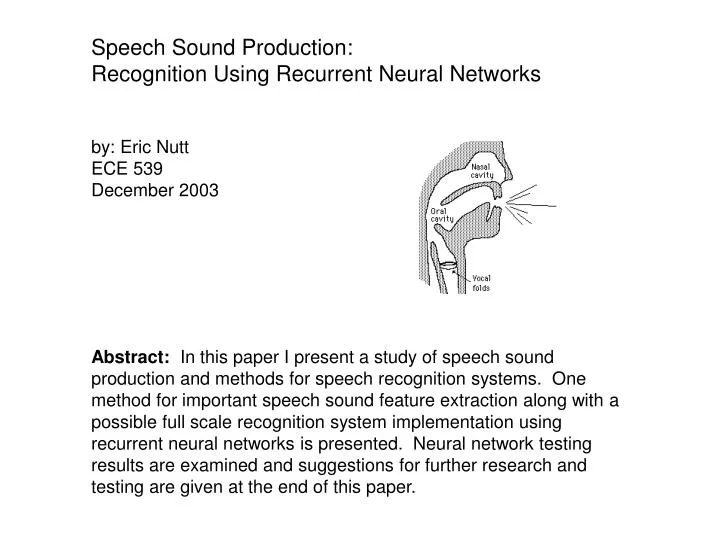
Speech Sound Production: Recognition Using Recurrent Neural Networks. by: Eric Nutt ECE 539 December 2003.

E N D
Speech Sound Production: Recognition Using Recurrent Neural Networks by: Eric Nutt ECE 539 December 2003 Abstract: In this paper I present a study of speech sound production and methods for speech recognition systems. One method for important speech sound feature extraction along with a possible full scale recognition system implementation using recurrent neural networks is presented. Neural network testing results are examined and suggestions for further research and testing are given at the end of this paper.
Nasal Cavity Throat Mouth Lungs Diaphragm Processes controlling speech production: Phonation: converting air pressure into sound via the vocal folds Resonation: emphasizing certain frequencies by resonances in the vocal tract Articulation: changing vocal tract resonances to produce distinguishable sounds Speech Sound Mechanisms Anatomy responsible for speech production: Cavity Resonator Air forced up from the lungs by the diaphragm passes through the vocal folds at the base of the larynx. Sound is produced by vibrations of the vocal folds and then the sound is filtered by the rest of the vocal tract. This sound production system acts much like that of a cavity resonator where the resonant frequency is given by:
Phonology The study of phonemes, the smallest distinguishable speech sounds. Phonemes can be separated in different ways but one common way is by the manner of articulation. This method breaks phonemes into groups based on location/shape of vocal articulators. One of the most important properties of a particular phoneme is its voicing. If the vocal folds are used to produce the sound then it is said to be voiced, otherwise it is not voiced. Articulators: lip opening, shape of the body of the tongue, and the location of the tip of the tongue Phoneme groups: Fricatives: constant restriction of airflow [f] as in foot and [v] as in view Stops: complete restriction of airflow followed by a release [p] as in pie and [b] as in buy Affricates: stop followed by a fricative [č] as in chalk and [ ĵ] as in gin Example of an voiced fricative /v/ Example of an unvoiced fricative /s/ Waveform and Spectrum of /s/ Waveform and Spectrum of /v/
Speech Waveform Windowing |FFT|2 Logarithm Mel Filter Bank DCT MFCC Speech Feature Extraction • Record Speech Waveform @ 20 kHz because human speech • reaches only about 10 kHz. • 2. Select small section (20 to 30 ms) representing the phone • of interest. • Break into 100 or more overlapping sections and apply a • Hamming Window to each section • Calculate 256 point |FFT|² power spectrum of each section. • Discard phase information because studies show perception • is based on magnitude. • Take the logarithm because humans hear loudness on an • approximately log scale. • Apply a Mel-Frequency Filter Bank to enhance perceptually • important frequencies and reduce feature dimensions. • Average over time to reduce the time dimensions. • Take Discrete Cosine Transform of time averaged spectrum in • order to produce Mel-Frequency Cepstral Coefficients. Keep the first • 13 to 15 coefficients as they contain nearly all of the energy of the • spectrum.
F37 F38 F39 F40 … Mel-Filter bank Purpose: Enhance perceptually important frequencies and reduce feature size by applying a bank of filters to each spectrum. Making the filter bank: Take about 40 linearly spaced points in the Mel-frequency scale and convert to the regular frequency scale using: Use these points as the peaks for each filter. Applying the filter bank: Multiply each filter by the spectrum values in the spectrum index range covered by that filter. Sum up the results. Result: After doing this the spectrum dimension will be reduced to the number of filters in the filter bank. The lower frequencies will be filtered at a higher resolution in order to enhance these perceptually more important frequencies.
Neural Network Recognition Intro: Neural networks are an obvious choice for speech recognition as a result of their ability to classify patterns. One important thing to note about classifying phonemes is that each phone has a feature vector that is really a sequence of vectors (or a matrix) with the rows representing the Mel-Frequency Cepstral Coefficients and the columns representing time. Acoustic-Phonetic Recognition System: This system is based on distinguishing phonemes by their acoustic properties. Feature vectors (phone/acoustic vectors) are gathered and introduced in parallel to expert networks that are each trained to recognize a particular phoneme. The complete output is recorded over time to get phoneme hypotheses which are then stochastically processed to decide the closest matching word. The Experts: In order to process feature vectors that depend on time a recurrent network should be used because they have memory (current outputs depend on past inputs). One could use an Elman or Jordan network to accomplish such a task. A Slightly modified back-propagation algorithm can be used to train networks like these.
Neural Network Testing and Results In all 5 networks were trained to recognize the phoneme /s/. First 25 samples were gathered and split into a training set (20 samples) and a test set (5 samples). The testing consisted of the following steps: • Training set randomly ordered and current network structure trained for 3000 epochs. • The training algorithm used was a back-propagation steepest descent algorithm with • adaptive learning rate and momentum. Trained network then used to classify training set • and test set to get training and testing error (in terms of percent missed). • 2. Five trials of step 1 were done and averaged for each network. • 3. Step 2 repeated four times with different training parameters (initial learning rate • and momentum constant) each time. • 4. The results were tallied: Conclusion: The network structure that learned /s/ the best is the [16,8,1] structure. This network had 2 fully connected recurrent layers with 16 and 8 neurons and one output layer with 1 neuron. Although this network had the second best training error at 22% (next to the [16,4,1] structure with 19%) it had a much lower testing error at 80% (versus 90% for the other network). With these testing error results I have determined that a lot more data and time is required to obtain decent testing errors (maybe around 20 to 30%).