Download

1 / 12
140 likes | 161 Views
AI: Neural Networks lecture 5 Tony Allen School of Computing & Informatics Nottingham Trent University. Recurrent Neural Networks. The solution to many real world problems require information concerning past inputs.

E N D
AI: Neural Networks lecture 5Tony AllenSchool of Computing & InformaticsNottingham Trent University
Recurrent Neural Networks The solution to many real world problems require information concerning past inputs. Recurrent neural networks are ones in which the output node (or hidden node) activations from one time step are feed back to form all or part of the input node activations for the next time step. Such networks are capable of learning sequential or time-varying patterns.
SRN Training Algorithm The training algorithm for the simple recurrent network is as follows: 1. Set activations of context units to 0.5 2. Do steps 3 – 7 until end of training set 3. Present current input vector to inputs X1 – Xn 4. Calculate predicted next output vector Z1 - Zn 5. Compare predicted output to target output vector 6. Determine error, back-propagate, update weights 7. Test for stopping condition: if stopping condition = true then stop else copy activations of hidden units to context units C1 – Cn and continue Information processing is sequential in time, so feed-forward, backpropagation & weight updating algorithms are essentially the same as for a standard back-propagation network.
SRN for finite-state grammar validation One example of the use of a simple recurrent network is for predicting the next letter in a string of characters. The strings are generated bya small finite-state grammar in which each letter appears twice, followed by a different character. Each string begins with the symbol B and ends with the symbol E. Valid string = B P V V E Invalid string = B T X P V E
SRN Architecture For the context-sensitive grammar shown on the previous slide, each input and output vector would be represented by a 6 component vector i.e. B = 1,0,0,0,0,0 T = 0,0,0,1,0,0 & E = 1,0,0,0,0,0 The SRN would thus have six input units (one for each of the five characters, plus one for the Begin symbol) and six output units (one for each of the five characters, plus one for the End symbol). There are three hidden units and therefore three context units C1 – C3.
Training Algorithm The training algorithm for the context-sensitive grammar problem is as follows: 1. Set activations of context units to 0.52. Do steps 3 – 7 until end of String 3. Present current symbol to inputs X1 – X6 4. Present next symbol to outputs as target vector 5. Calculate predicted next symbol 6. Determine error, back-propagate, update weights 7. Test for stopping condition If target = E then stop else copy activations of hidden units to context units C1 – C3 and continue
Specific example Suppose the string B T X S E is used for training: 1. Begin training for this string a. X1 – X6 = 1,0,0,0,0,0 (B) b. Z1 – Z6 = 0,0,0,1,0,0 (T) c. Compute predicted response d. Determine error, back-propagate, update weights e. C1 – C3 = Y1 – Y32. Training for second symbol in string a. X1 – X6 = 0,0,0,1,0,0 (T) b. Z1 – Z6 = 0,0,0,0,0,1 (X) c. Compute predicted response d. Determine error, back-propagate, update weights e. C1 – C3 = Y1 – Y3
Specific example cont. 3. Training for third symbol in string a. X1 – X6 = 0,0,0,0,0,1 (X) b. Z1 – Z6 = 0,1,0,0,0,0 (S) c. Compute predicted response d. Determine error, back-propagate, update weights e. C1 – C3 = Y1 – Y34. Training for fourth symbol in string a. X1 – X6 = 0,1,0,0,0,0 (S) b. Z1 – Z6 = 1,0,0,0,0,0 (E) c. Compute predicted response d. Determine error, back-propagate, update weights e. Target response is the End symbol therefore training is complete for this string.
Generalisation After training, the net can be used to determine whether or not a string is valid according to the grammar specified. As each symbol is presented, the network predicts the possible valid successors to the current input symbol. Any output unit with an activation of 0.3 or greater is then taken to indicate that the letter it represents is a valid successor to the current input. To determine whether or not a string is valid, the letters are presented to sequentially to the network for as long as the network continues to predict valid successors in the string. If the net fails to predict a successor, the string is rejected. If all successors are predicted then the string is accepted as valid.
Simple Recurrent Network • The simple recurrent network can be used to learn to predict the next words in sentences generated using a simple grammar. • In this case: • X1 – Xn represents the current word input vector applied to the network at time t • Target output is the t+1 word vector in training sentence. • C1 – Cn represents the information feedback from the hidden units at time step t-1. • The weights on the feedback connections to the context units are fixed at 1. http://crl.ucsd.edu/~elman/Papers/fsit.pdf
SRN: Finding structure in time For the simple grammar described each input and output vector is represented by a 31 component vector i.e. man 0000000000000000000000000000010 smash 0000000000000000000000000010000 plate 0000000000000000000001000000000 The SRN thus had 31 input units & 31 output units. There were 150 hidden units and therefore 150 context units. The network was trained over 6 epochs of a 27,354 word training set. After training, the network was found to have developed internal (hidden unit) representations for the input vectors that reflected facts about the possible sequential ordering of the input vectors - animate noun precedes verb precedes inanimate noun.
References Servan-Schreiber, D., A. Cleeremans, & J. L. McClelland. (1989). “Learning Sequential Structure in Simple Recurrent Networks.” In D. S. Toutetzky, ed., Advances in Neural Information Processing Systems 1. San Mateo, CA: Morgan Kaufmann, pp. 643-652. Elman, J. L (1990). “Finding Structure in Time” Cognitive Science, 14: 179-211.