Download
1 / 28
300 likes | 488 Views
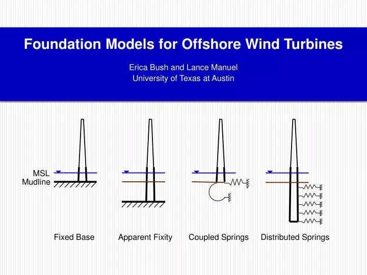
Foundation Models for Offshore Wind Turbines Erica Bush and Lance Manuel University of Texas at Austin. MSL. Mudline. Fixed Base. Apparent Fixity. Coupled Springs. Distributed Springs. Problem Overview.

E N D
Foundation Models for Offshore Wind Turbines Erica Bush and Lance Manuel University of Texas at Austin MSL Mudline Fixed Base Apparent Fixity Coupled Springs Distributed Springs
Problem Overview • Characteristic loads for reliability-based design of offshore wind turbines can be derived from time-domain aeroelastic-hydrodynamic response simulations Design load = Load Factor × Characteristic Load • Accuracy of derived characteristic loads depends on • number of simulations run • accuracy of critical sea state selection (when using Inverse FORM) • accuracy of the simulation models used • ObjectiveCompare loads derived from alternative foundation model using simulations
Wind Turbine Model Outer diameter = 3.87 m Wall thickness = 1.9 cm Hub • 5 MW baseline offshore wind turbine developed at the National Renewable Energy Laboratory (NREL) • 11.5 m/s rated wind speed • FAST is used to simulate waves and turbine response; TurbSim is used to simulate wind Tapers linearly upward Outer diameter = 6 m Wall thickness = 2.7 cm 126 m MSL Outer diameter = 6 m Wall thickness = 6 cm Mudline 90 m 20 m not to scale 36 m
Foundation Models MSL Mudline Fixed Base Apparent Fixity Coupled Springs Distributed Springs Different properties and dimensions need to be specified for each model These properties and dimensions depend on the sea state considered We discuss how they are computed and then used in FAST
Apparent Fixity Model Ѳ Ѳ M M M F F w w F AFL, EI 36 m STEP 3 STEP 1 STEP 2 From a fixed base simulation, obtain shear, F, and moment, M, values at the mudline in the fore-aft direction
Apparent Fixity Model Ѳ Ѳ M M M F F w w F AFL, EI 36 m STEP 3 STEP 1 STEP 2 Determine the corresponding deflection, w, and rotation, Ѳ, for the real pile
Apparent Fixity Model Ѳ Ѳ M M M F F w w F AFL, EI 36 m STEP 3 STEP 1 STEP 2 Calculate the length and stiffness of a cantilever that would produce the same deflection and rotation for the given shear and moment
Step 1: Shear and Moment Values For each sea state, 50 contemporaneous shear (F) and moment (M) pairs at the tower base in the fore-aft direction are randomly selected from a single fixed base simulation idea: to calibrate flexible foundation model for anticipated loads from what’s above the mudline Are 50 random pairs selected from one fixed-base simulation representative?
Step 2: Deflections and Rotations Sand 1 γ = 10 kN/m3 Ф’ = 33° k = 16287 kN/m3 5 m Sand 2 γ = 10 kN/m3 Ф’ = 35° k = 24430 kN/m3 9 m γ = 10 kN/m3 Ф’ = 38.5° k = 35288 kN/m3 Sand 3 22 m • We use LPILE to perform lateral pile analysis (with p-y curves) in order to determine the deflections and rotations of the real pile based on each of the shear and moment pairs • The p-y curves for the lateral force-displacement relationships are based on API guidelines • A pile length of 36 m below the mudline and this sand profile were chosen based on previous work (Passon, 2006; Jonkman et al., 2007) Soil Profile Considered
Step 3: Equivalent Length and Stiffness M F L, EI L, EI L = AFL EI = Stiffness • L and EI are calculated for each of the 50 randomly selected shear and moment pairs • The average L and EI is then used in the model
Coupled Springs Model • Spring stiffnesses are calculated from the AFL and EI Flexibility Matrix Stiffness Matrix
Coupled Springs Model wind heave sway yaw pitch surge roll • Note that the AFL and EI were calculated from shear and moment in the fore-aft direction • But the translational and rotational springs will be attached in both horizontal directions (totaling four coupled springs) • Heave and yaw DOF are turned off • FAST must be recompiled with this platform stiffness matrix
Distributed Springs Model • The sea state must be represented by a single shear and moment pair • The shear and moment pair that has an AFL closest to the average AFL is selected from the 50 contemporaneous pairs . . . Note: V = 12 m/s is shown in table
Distributed Springs Model . . . LPILE is run with the chosen shear and moment pair We discretize the embedded pile at 252 points; LPILE gives the distributed lateral resistance and deflection at each point The lateral spring stiffness is calculated at each point by dividing the distributed resistance (kN/m) by the deflection (m) and, then, multiplying by the tributary length (m) for that point result: spring stiffness for each point in kN/m We reduce the number of springs to 37 at 1-meter spacing by adding stiffnesses at points within the tributary length of each discrete spring FAST is recompiled with these spring stiffnesses for each simulation with the distributed springs model
w u v Loading Models Wind load Wave load • Random wind loading • 3-D Inflow turbulence random field over a 2-D rotor plane uses Kaimal power spectrum and exponential coherence spectrum • Random wave loading • Irregular long-crested waves are simulated using a JONSWAP spectrum, Airy wave kinematics, and Morison’s equation • Structural response • Combine modal and multi-body dynamics formulation (includes control systems)
Selecting Critical Sea States • 2D Inverse FORM (Environmental Contour Method) U2 Rosenblatt Transformation U1 (-) = PT= Target Failure Probability = Reliability index • 20-year return period considered (T = 20 yrs) • PT = 1/(20 × 365.25 × 24 × 6) = 9.51 × 10⁻⁷ (load exceedance probability in 10 mins) b = 4.76
Summary Statistics ( V = 12 vs. 22 m/s) Fore-Aft Tower Bending Moment at the Mudline for Fixed Base Model (150 sims) Fore-Aft Tower Bending Moment at the Mudline for Apparent Fixity Model (150 sims) Mean + (Std. Dev.)(PF) = Max +x = Going from 12 to 22 m/s (with either fixed base or AF model)
Summary Statistics (Fixed vs. Flexible) Fore-Aft Tower Bending Moment at the Mudline for Fixed Base Model (150 sims) Fore-Aft Tower Bending Moment at the Mudline for Apparent Fixity Model (150 sims) Consider 12 m/s sea state only With change from fixed-base to flexible model Mean is unchanged; SD increases by ~20%, PF is unchanged; hence max increases but by only ~10% [since max = mean + SD × PF]
Summary Statistics Fore-Aft Tower Bending Moment at the Mudline for V = 12 m/s (150 sims) Max = Mean + (Std. Dev.)(PF) • Mean trend matches control system’s dependence on mean wind speed • All models are seeing the same wind and wave time series; so, control system behaves the same way as far as mean load goes • Only about 3% difference between largest and smallest mean (among models)
Summary Statistics Fore-Aft Tower Bending Moment at the Mudline for V = 12 m/s (150 sims) Max = Mean + (Std. Dev.)(PF) wind structure TBM f f f
Summary Statistics Fore-Aft Tower Bending Moment at the Mudline for V = 12 m/s (150 sims) Max = Mean + (Std. Dev.)(PF) • PF = f(exposure time, asymmetry, tails, upcrossing rate) • Only about 4% difference between flexible foundation models
Summary Statistics Fore-Aft Tower Bending Moment at the Mudline for V = 12 m/s (150 sims) Max = Mean + (Std. Dev.)(PF) • The variability in maxima for the four models mostly depends on std. dev. • As std. dev. increases, the max increases
Power Spectra • High frequency peaks shift left as the upcrossing rate for the model decreases • AF and CS have very similar behavior because they tell FAST effectively the same information • However, the AF model has more inertia by design • AF has slightly less power than CS as seen in the smaller std. dev.
Exceedance Plots Median of 10-min. Extremes (MN-m) • Median of 10-min. extreme can be taken as 20-year characteristic value (Inverse FORM) • 20-year loads for the flexible models differ by less than 6% (from each other) • All four models have 90% confidence interval < 4 MN-m (on 20-year load) based on bootstrap estimation • 150 simulations are sufficient for 2D Inverse FORM • Tails will be more important for 3D Inverse FORM • Then, more simulations will be necessary
Another Sea State Median of 10-min. Extremes (MN-m) Fore-Aft Tower Bending Moment at the Mudline for V = 22 m/s (150 sims) • Medians of 10-min. extremes for this sea state are not associated with 20-year load because they are not the largest on the environmental contour • Medians for the three flexible models differ by less than 1% (from each other) • Statistics and power spectra have similar trends to the 12 m/s case
Recipe for Use of Flexible Foundation Models • Each sea state requires the following steps: STEP 1 Run one fixed base simulation, and select 50 random shear and moment pairs from the time series. STEP 2 Run LPILE for all 50 load pairs, and calculate the AFL and EI for each pair. STEP 3AF modelUse the average AFL and EI. CS model Use the average AFL and EI to calculate the coupled spring constants. DS model Choose the shear and moment pair that produces an AFL and EI closest to the average. Run LPILE for this pair, and calculate distributed spring constants from the output. STEP 4 Run N simulations per model, and extract N 10-min extremes. (N = 150 was used here apply Inverse FORM to get long-term load)
Conclusions • The three flexible models yield 20-year loads that are within 6% of each other when using 2D Inverse FORM to evaluate critical sea states • The three flexible models seem fairly interchangeable, but AF may be the easiest to implement because FAST does not need to be recompiled Future Work • The AF and CS models do not have same mass as the original structure • Evaluate alternative inertia distributions for these • Verify whether 50 random (F, M) pairs from a single FB simulation are sufficient • Perform 3D Inverse FORM (a more accurate approach to sea state selection) • Well-behaved tails are required for acceptable confidence in 20-year loads • More simulations are necessary to produce well behaved tails • Study other soil profiles to evaluate flexible foundation models
Acknowledgments • Dr. Jason Jonkman of the National Renewable Energy Laboratory • Dr. Puneet Agarwal, former student of Dr. Lance Manuel • Dr. Shin Tower Wang of Ensoft, Inc. • National Science Foundation Grant No. CMMI-0449128 (CAREER) Grant No. CMMI-0727989