Download
1 / 37
370 likes | 374 Views
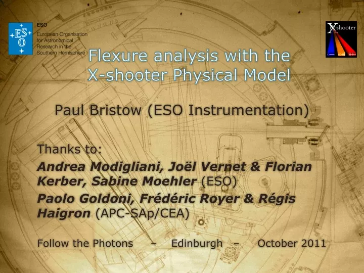
Flexure analysis with the X-shooter Physical Model. Paul Bristow (ESO Instrumentation) Thanks to: Andrea Modigliani, Joël Vernet & Florian Kerber, Sabine Moehler (ESO) Paolo Goldoni, Frédéric Royer & Régis Haigron (APC-SAp/CEA) Follow the Photons – Edinburgh – October 2011.

E N D
Flexure analysis with theX-shooter Physical Model Paul Bristow (ESO Instrumentation) Thanks to: Andrea Modigliani, Joël Vernet & Florian Kerber, Sabine Moehler (ESO) Paolo Goldoni, Frédéric Royer & Régis Haigron (APC-SAp/CEA) Follow the Photons – Edinburgh – October 2011
Matrix Representation of Optics • ME is the matrix representation of the order m transformation performed by an Echelle grating with E at off-blaze angle . This operates on a 4D vector with components (wavelength, x, y, z).
Applications • Wavelength calibration • Simulations • Early DRS development • Effects of modifications/upgrades • Instrument monitoring/QC • Advanced ETC?
Some background • M. Rosa: Predictive calibration strategies: The FOS as a case study (1995) • P. Ballester, M. Rosa: Modeling echelle spectrographs (A&AS 126, 563, 1997) • P. Ballester, M. Rosa: Instrument Modelling in Observational Astronomy (ADASS XIII, 2004) • Bristow, Kerber, Rosa: four papers in HST Calibration Workshop, 2006 • UVES, SINFONI, FOS, STIS, CRIRES,X-shooter – Bristow et al (Experimental Astronomy 31, 131, 2011)
X-Shooter (300nm-2.5m) • Commissioned 2009 • Vernet et al. 2011.A & A. in press • Model for UVB, VIS& NIR arms • Same model kernel • Independent configuration files • Cross dispersed, medium res’n, single slit • Single mode (no moving components) • Cassegrain & heavy => Flexure
X-shooter Flexure • Backbone flexure • Causes movement of target on spectrograph slits • Corrected with Automatic Flexure Compensation exposures • Spectrograph flexure • Flexing of spectrograph optical bench • Can also be measured in AFC exposures • First order translation automatically removed by pipeline UVB VIS NIR
Lab Measurements • NIR arm • Multi-pinhole • Translational & higher order distortions
AFC Exposures • Obtained with every science obs => large dataset ~300 exp from Jan – May 2011 • Single pinhole, Pen-ray lamp • Window: • 1000x1000 win (UVB 12/VIS 14 lines) • Entire array (NIR 160 lines) VIS UVB NIR
Physical Model Optimisation FOR EVERY CALIBRATION EXPOSURE
Choosing “open” parameters • All parameters open • Slow • Optimal result • Degeneracy • Physically motivated: • Related to flexure • Constrained by data • In these results: • Prism orientation; Grating Orientation; Grating constant; Camera focal length; Detector position and orientation
NIR (Product moment correlation)
Summary • Simple physical modelling approach: • wavelength calibration for a number of instruments • Raw data simulation • Instrument monitoring • Application to X-shooter • Flexure monitoring • Allows identification of physical model parameters that correlate with instrument orientation
Physical Model Optimisation • QC Data • 9 pinhole mask, arc lamp: • Th-Ar (UVB 250 lines x 9 & VIS 390 lines x 9) • pen-ray (NIR 140 lines x 9) • Daytime, Zenith (no flexure except hysteresis) • 1/week => small data set • Automatically processed by pipeline (ESO QC)
Effective camera focal length (mm) Effective camera focal length (mm) UVB Camera temperature sensor reading (°C) VIS Camera temperature sensor reading (°C)
Detector tilt (°) Detector tip (°) Effective camerafocal length (mm) Modified Julian Date (days)
Explain “our Physical Models” • Compare to poly • Uses • Calibration • Simulation • Test DRS • Investigate modifications/upgrades • Monitor/understand instrument behaviour • History (Ballester & Rosa) • Introduce X-shooter • Overview • Flexure • Lab plots • AFC • Calibration exposures • Flexure Procedure • Optimisation for 1 exposure • Apply to all data • Choosing open parameters • Flexure Results • NIR • Residuals • Sin plot • Linear plots • Table – highlight interesting param combinations • UVB • Residuals • Linear plots • table • VIS • Residuals • Linear plots • table • Flexure conclusions • QC • Procedure • Results • Summary