Unsupervised Learning Clustering & Dimensionality Reduction 273A Intro Machine Learning

1. Unsupervised Learning Clustering & Dimensionality Reduction 273A Intro Machine Learning

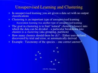
2. What is Unsupervised Learning? • In supervised learning we were given attributes & targets (e.g. class labels). • In unsupervised learning we are only given attributes. • Our task is to discover structure in the data. • Example I: the data may be structured in clusters: • Example II: the data may live on a • lower dimensional manifold: Is this a good clustering?

3. Why Discover Structure ? • Data compression: If you have a good model you can encode the • data more cheaply. • Example: To encode the data I have • to encode the x and y position of each data-case. • However, I could also encode the offset and angle • of the line plus the deviations from the line. • Small numbers can be encoded more cheaply than • large numbers with the same precision. • This idea is the basis for model selection: • The complexity of your model (e.g. the number of parameters) should be • such that you can encode the data-set with the fewest number of bits • (up to a certain precision).

4. the a on ... 5 4 7 0 0 0 1 3 5 0 0 0 0 0 0 1 0 0 0 4 0 0 1 ... Why Discover Structure ? • Often, the result of an unsupervised learning algorithm is a new representation • for the same data. This new representation should be more meaningful • and could be used for further processing (e.g. classification). • Example I: Clustering. The new representation is now given by the label of a • cluster to which the data-point belongs. This tells us how similar data-cases are. • Example II: Dimensionality Reduction. Instead of a 100 dimensional vector • of real numbers, the data are now represented by a 2 dimensional vector • which can be drawn in the plane. • The new representation is smaller and hence more convenient computationally. • Example I: A text corpus has about 1M documents. Each document is represented • as a 20,000 dimensional count vector for each word in the vocabulary. • Dimensionality reduction turns this into a (say) 50 dimensional vector for each doc. • However: in the new representation documents which are on the same topic, • but do not necessarily share keywords have moved closer together!

5. Clustering: K-means • We iterate two operations: • 1. Update the assignment of data-cases to clusters • 2. Update the location of the cluster. • Denote the assignment of data-case “i” to cluster “c”. • Denote the position of cluster “c” in a d-dimensional space. • Denote the location of data-case i • Then iterate until convergence: • 1. For each data-case, compute distances to each cluster and the closest one: • 2. For each cluster location, compute the mean location of all data-cases • assigned to it: Nr. of data-cases in cluster c Set of data-cases assigned to cluster c

6. K-means • Cost function: • Each step in k-means decreases this cost function. • Often initialization is very important since there are very many local minima in C. • Relatively good initialization: place cluster locations on K randomly chosen data-cases. • How to choose K? • Add complexity term: and minimize also over K • Or X-validation • Or Bayesian methods

7. Vector Quantization • K-means divides the space up in a Voronoi tesselation. • Every point on a tile is summarized by the code-book vector “+”. • This clearly allows for data compression !

8. Mixtures of Gaussians • K-means assigns each data-case to exactly 1 cluster. But what if • clusters are overlapping? • Maybe we are uncertain as to which cluster it really belongs. • The mixtures of Gaussians algorithm assigns data-cases to cluster with • a certain probability.

9. MoG Clustering Covariance determines the shape of these contours • Idea: fit these Gaussian densities to the data, one per cluster.

10. EM Algorithm: E-step • “r” is the probability that data-case “i” belongs to cluster “c”. • is the a priori probability of being assigned to cluster “c”. • Note that if the Gaussian has high probability on data-case “i” • (i.e. the bell-shape is on top of the data-case) then it claims high • responsibility for this data-case. • The denominator is just to normalize all responsibilities to 1:

11. EM Algorithm: M-Step total responsibility claimed by cluster “c” expected fraction of data-cases assigned to this cluster weighted sample mean where every data-case is weighted according to the probability that it belongs to that cluster. weighted sample covariance

12. EM-MoG • EM comes from “expectation maximization”. We won’t go through the derivation. • If we are forced to decide, we should assign a data-case to the cluster which • claims highest responsibility. • For a new data-case, we should compute responsibilities as in the E-step • and pick the cluster with the largest responsibility. • E and M steps should be iterated until convergence (which is guaranteed). • Every step increases the following objective function (which is the total • log-probability of the data under the model we are learning):

13. Dimensionality Reduction • Instead of organized in clusters, the data may be approximately lying on a • (perhaps curved) manifold. • Most information in the data would be retained if we project the data on this • low dimensional manifold. • Advantages: visualization, extracting meaning attributes, computational efficiency

14. Principal Components Analysis • We search for those directions in space that have the highest variance. • We then project the data onto the subspace of highest variance. • This structure is encoded in the sample co-variance of the data:

15. 0 0 PCA • We want to find the eigenvectors and eigenvalues of this covariance: ( in matlab [U,L]=eig(C) ) eigenvalue = variance in direction eigenvector Orthogonal, unit-length eigenvectors.

16. 0 0 PCA properties (U eigevectors) (u orthonormal  U rotation) (rank-k approximation) (projection)

17. PCA properties is the optimal rank-k approximation of C in Frobenius norm. I.e. it minimizes the cost-function: Note that there are infinite solutions that minimize this norm. If A is a solution, then is also a solution. The solution provided by PCA is unique because U is orthogonal and ordered by largest eigenvalue. Solution is also nested: if I solve for a rank-k+1 approximation, I will find that the first k eigenvectors are those found by an rank-k approximation (etc.)