Download
1 / 228
2.36k likes | 2.44k Views
Decomposition of Graph. Decomposition of Graph In the remaining of this chapter, we will cover graphs, including Depth-First Search, and Breadth-First Search, and Topological Sorting. Graphs: A graph G = (V, E) is defined by a pair of two sets:

E N D
Decomposition of Graph • In the remaining of this chapter, we will cover • graphs, including • Depth-First Search, and • Breadth-First Search, and • Topological Sorting
Graphs: • A graph G = (V, E) is defined by a pair of two sets: • V is a finite set of vertices (nodes) and • E is a set of pairs of vertices, called edges. • A graph G is called undirectedif every edge in it is undirected. • This definition yields an undirected graph that • disallows multiple edges between the same vertices • every pair of vertices, u and v is unordered, i.e., • a pair of vertices (u, v) is the same as the pair (v, u), • the vertices u and v are adjacent to each other and • they are connected by the undirected edge (u, v).
We said that • the vertices u and v are endpoints of the edge(u, v); • u and v are incident to this edge; • the edge (u, v) is incident to its endpoints u and v.
Directed graph • A directed graph (also called a digraph) is a graph whose every edge is directed. • If a pair of vertices (u, v) is not the same as the pair (v, u) we say that the edge (u, v) is directed from the vertex u, called the edge’s tail, to the vertex v, called the edge’s head. [We can omit .] • We also say that the edge (u, v) leaves u and enters v. u v
Given an undirected graph G = (V, E), the following inequality for the number of edges |E| which is possible in the undirected graph with |V| vertices and no loops (self-loop?): • 0 ≤ |E| ≤ |V| (|V| - 1). • Example 3.4: • Let the number of vertices |V| = 6. • The max number of edges |E| = (|V| * |V-1|) = (6 * 5 ) = 15. • a c b • d e f
A graph with every pair of its vertices connected by an edge is called complete. • K|V|is used to denote a complete graph with |V| vertices. • A graph with relatively few possible edges missing is called dense. • A graph with few edges relative to the number of its vertices is called sparse.
Example 3.5: Let G = (V, E) be an undirected graph where V = { a, b, c, d, e, f} E = {(a, c), (a, d), (b, c), (b, f), (c, e), (d, e), (e, f)} a c b d e f It is not a complete graph since not every pair of vertices is connected by an edge; for example, there is no edge between a and b, between c and d, etc.
Example 3.6: Let G = (V, E) be a digraph, where V = { a, b, c, d, e, f} E = {(a, c), (b, c), (b, f), (c, e), (d, a), (d, e), (e, c), (e, f)} a c b d e f
Graph representation • Graphs for computer algorithm can be represented in two ways: • the adjacency matrix and • adjacency lists.
A graph or digraph can be represented by an adjacency matrix; if there are n = |V| vertices v1, v2, …, vn, this is an n x n array whose (irow, jcol)thentry is • 1 if there is an edge from vi to vj, • aij = • 0 otherwise. • The adjacency matrix of a graph with n vertices is an n-by-n Boolean matrix with one row and one column for each of the graph’s vertices. • 1 isin (irow, jcol)th entry if there is an edge from the vertex i to thevertex j, and • 0 is in (irow, jcol)th entry if there is no such edge.
Example 3.5: An adjacency matrix for the undirected graph G. Let G = (V, E) be an undirected graph where V = { a, b, c, d, e, f} E = {(a, c), (a, d), (b, c), (b, f), (c, e), (d, e), (e, f)} a c b d e f
Example 3.6: Let G = (V, E) be a digraph, where V = { a, b, c, d, e, f} E = {(a, c), (b, c), (b, f), (c, e), (d, a), (d, e), (e, c), (e, f)} a c b d e f
The adjacency matrix of an undirected graph with n vertices: • The presence of a particular edge can be checked in constant time Θ(1), with just one memory access. (is the entry of ith row and jth column A[i, j] = 1.) • But the matrix takes up O(n2) space, which is wasteful if the graph does not have very many edges.
The adjacency lists of a graph or a digraph is a collection of linked lists one for each vertex, that contain all the vertices adjacent to the list’s vertex (i.e., all the vertices connected to it by an edge). The following adjacency lists is of the graph in Example 3.5.
Example 3.5: An adjacency list for the undirected graph G Let G = (V, E) be an undirected graph where V = { a, b, c, d, e, f} E = {(a, c), (a, d), (b, c), (b, f), (c, e), (d, e), (e, f)} a c b d e f
Example 3.6: Let G = (V, E) be a digraph, where V = { a, b, c, d, e, f} E = {(a, c), (b, c), (b, f), (c, e), (d, a), (d, e), (e, c), (e, f)} a c b d e f
The adjacency-list consists of |V| linked lists, one per vertex. • For a directgraph, each edge appears in exactly one of the linked lists. • For an undirectedgraph, each edge is represented by two of the lists. • For undirected graphs, this representation has a symmetry of sorts: v is in u’s adjacency list if and only if u is in v’s adjacency list. • The total size of the data structure is O(|E|) for either way. • Checking for a particular edge (u, v) for a digraph is no longer constant time, because it requires sifting through u’s adjacency list. But it is easy to iterate through all neighbors of a vertex (by running down the corresponding linked list). But the matrix takes up O(n2) space O(|V|)
Two representations of a directed graph G with 6 vertices and 9 edges: • An adjacency-list representation of G. • An adjacency-matrix representation of G.
Example 3.6: An adjacency-list representation of a digraph G. Let G = (V, E) be a digraph, where V = { a, b, c, d, e, f} E = {(a, a) (a, c), (b, c), (b, f), (c, e), (d, a), (d, e), (e, c), (e, f)} c a b f d e What is the best data structure needed to support DFS and BFS?
Example 3.6: An adjacency-matrix representation of a digraph G. Let G = (V, E) be a digraph, where V = { a, b, c, d, e, f} E = {(a, a), (a, c), (b, c), (b, f), (c, e), (d, a), (d, e), (e, c), (e, f)} What is the best data structure needed to support DFS and BFS? c a b f d e
Weighted graphs • A weighted graph (or weighted digraph) is a graph (or digraph) with numbers (called weights or costs) assigned to its edges. • Both adjacency-list and adjacency-matrix representations of a graph can be extended to accommodate weighted graphs. • For a weighted graph which is represented by its adjacency-matrix, its element A[i, j] will simply contain • the weight of the edge from the ith vertex to the jthvertex if there is such an edge and • a special symbol, e.g., ∞, there is no such edge. • Such a matrix is called the weight matrix or cost matrix. c
c Example 3.5a of a weighted graph a 5 b 1 4 c 2 d 7 The weight matrix or cost matrix. 7
Paths, Cycles, Connectivity and Acyclicity. • Apathfrom vertex u to vertex v of a graph G can be defined as a sequence of adjacent (connected by an edge) vertices that starts with u and ends with v. • p = { u = u0, u1, u2, … , un = v | for all ui, ui+1 ε V and (ui, ui+1) ε E} • Thelengthof a path is the total number of vertices in a vertex sequence defining the path minus one, (|V| - 1), which is the same as the number of edges in the path. c
The path contains the vertices u = u0, u1, u2, … , un = v and the edges (u0, u1), (u1 , u2 ), …, (un-1, un ). • There is always a 0-length path from u to u. • If there is a path p from u to v, we say that v is reachable from u via p, which we denote as u v if G is directed. • A path is said to be simple, if all vertices of a path are distinct • Psimple = { u = u0, u1, u2, … , un = v | for all ui, ui+1, uj ε V and • (ui, ui+1) ε E, ui, ≠ ui+1 ≠ uj }. c ui, ≠ ui+1 ≠ uj, ui, ≠ uj and ui+1 ≠ ujrule out a cyclic.
Example 3.5: Let G = (V, E) be an undirected graph where V = { a, b, c, d, e, f} E = {(a, c), (a, d), (b, c), (b, f), (c, e), (d, e), (e, f)} a c b d e f a, c, b, f is a simple pathof length 3 from a to f. a, c, e, c, b, f is a path (not simple)of length 5 from a to f. So as a, d, e, c, b, f, e is not a simple path for e appears twice.
Example 3.6: Let G = (V, E) be a digraph, where V = { a, b, c, d, e, f} E = {(a, a) (a, c), (b, c), (b, f), (c, e), (d, a), (d, e), (e, c), (e, f)} For example: In the directed graph, a, c, e, f is a directed path from a to f in the graph. c a b A directed path is a sequence of vertices in which every consecutive pair of the vertices is connectedby an edge directed from the vertex listed first to the vertex listed next. f d e
c A graph is said to be connected if for every pair of its vertices u and v there is a path from u to v. {Are there any difference between directed graph and undirected graph?} A subgraphof a given graph G = (V, E) is a graph G’ = (V’, E’) such that V’ (is a subset of) V and E’ E. Formally, a connected component is a maximal (not expandable via an inclusion of another vertex and an edge) connected subgraph of a given graph. Example: All the given graphs in our previous examples are connected.
Example 3.7 a f b c e g h d i a node k The graph is not connected because there is no path, for example, from a to f. However, it does have three disjoint connected regions, corresponding to the following sets of vertices: {a, b, c, d, e}, {f, g, h, i}, {k}. c k These regions are called connected components: each of them is a subgraph that is internally connected but has no edges to the remaining vertices of the other regions.
A cycle is a path <u = u0, u1, u2, … , un = v> of a positive length (i.e., is the path contains at least one edge) that starts and ends at the same vertex (that is u = v) [and does not traverse the same edge more than once]. The cycle is simpleif, in addition, u = u0, u1, u2, … , un = v are distinct. A graph with no cycles is said to be acyclic.
Example 3.7 a f b c e g h d i a node k k For example, the path < f, g, i, h, f > is a cycle. The paths < f, g, i, h, f >, < g, i, h, f, g> , < i, h, f, g, i> and < h, f, g, i, h > form the same cycle. These cycles are simple. The path < f, g, i, h, g, f > is not a simple cycle.
The graph has three connected components: {1, 2, 5}, {3, 6} and { 4 } An undirected graph is connected if it has exactly one connected component. c 6 5 4 3 2 1
Free Trees Before we investigate more about breadth-first trees, we shall give a concept of free trees. A free tree is a connected, acyclic, undirected graph. We often omit the adjective “free” when we say that a graph is a tree. If an undirected graph is acyclic but possibly disconnected, it is a forest, in which each of its connected components is a tree. Many algorithms that work for trees also work for forests.
Figure 3.7(b) A forest. The forest in the Figure is not a tree because it is not connected. Figure 3.7(a) A free tree.
Figure 3.7(c) A graph that contains a cycle and is therefore neither a tree nor a forest.
The following theorem captures important facts about free trees. • Theorem 3.6 (Properties of free trees) • Let G = (V, E) be an undirected graph. The following statements are equivalent. • G is a free tree. • Any two vertices in G are connected by a unique simple path. • G is connected, but if any edge is removed from E, the result graph is disconnected. • G is connected, and | E | = | V | - 1. • G is acyclic, and | E | = | V | - 1. • G is acyclic, but if any edge is added to E, the result graph contains a cycle.
Rooted Trees • In Theorem 3.6, it states an important properties of trees is the fact that • for every vertices in a tree, there always exists exactly one simple path from on these vertices to the other. • This property makes it possible to choose an arbitrary vertex in a free tree to be the root of the root tree.
Rooted Trees r Level 0 f e, f and g are siblings. e, f and g are children of d. d is the parents of e, f and g. c Level 1 u b 11 e g Level 2 d d 11 11 11 u c Level 3 CV CV CV g f e b r Level 4 CV CV Vertices in the enclosed region are descendants of c, which is an ancestor of each. Figure 3.7(c) A rooted tree. Figure 3.7(a) A free tree.
Rooted Trees • A rooted tree is a tree in which there is one vertex that is distinguished from others and is called the root. • The level of a vertex is the number of the edges along unique path between it and the root. • The depth of a vertex v is the length of the simple path from the rooted to v. • The height of a rooted tree is the maximum level of any vertex of the tree; • (i.e., the longest simple path from the root to a leaf) of any vertex of the tree.
Rooted Trees • Given the root r or any internal vertex v of a rooted tree, • the children of v are all those vertices that are adjacent to v and are one level farther away from the root than v. • If v is a child of u, then u is called theparentof v; and • two distinct vertices v and w that are both children of the same parent u are said siblings.
Rooted Trees In a tree T, given two distinct vertices u and v, if u lies on the unique path between v and the root, then u is anancestorof v and v is a descendant of u. The vertex itself is usually considered tis own ancestor; the set of ancestors that excludes the vertex itself is referred to as the set of proper ancestors. The proper descendants exclude the vertex u itself. All descendants of a vertex u with all the edges connecting them form the subtree of T rooted at that vertex u. A vertex with no children is called a leaf; a vertex with at least one child is called parental. All the leaf nodes are external nodes. The parental nodes are internal nodes.
Ordered Trees An ordered tree is a rooted tree in which all the children of each vertex are ordered. A binary tree is an ordered tree in which every vertex has no more than two children and each child is designated as either a left child or right child of its parent; a binary tree may also be empty. A full binary tree is a binary tree in which each parent has exactly two children. When a number assigned to each parental vertex is larger than all the numbers in its left subtree and smaller than all the numbers in it right subtree. Such trees are called binary search trees.
The predecessor and successor of a node X in a binary tree, assuming all keys are distinct? 12, 13, 17, 20, 24, 25, 27 30, 33 30 Inorder walks: 20 30 39 A binary tree and a full binary tree X 20 39 c 25 36 50 13 51 40 38 27 17 24 33 12 Successor(X) Predecessor(X)
The predecessor and successor of a node X in a binary tree, assuming all keys are distinct? 30 20 Predecessor(X) 50 c 28 55 24 48 23 25 21 A binary tree but not a full binary tree X Successor(X) 22
Depth-First Search and Breadth-First Search Algorithms • Viewed as applications of the decrease-by-one technique. • Doing their main job of visiting vertices and traversing edges of a graph.
Depth-First Search Depth-first search is a surprisingly versatile linear-time procedure that reveals a wealth of information about a graph. The most basic question it addresses is, What parts of the graph are reachable from a given vertex? To understand this task, consider a given graph, say in the form of an adjacency list. This representation offers just one basic operation: finding the neighbors of a vertex. With only this primitive, the reachability problem is rather like exploring a labyrinth. Given the following Figure 3.1, clearly you need to record some intermediate information during exploration. c
Figure 3.1: Exploring a graph is rather like navigating a maze. c
c E D A B I J G H C F L K In terms of reachability, this graph is equivalent to the given maze in Figure 3.1.
During exploration for any graph traversal, • Boolean variable : we need to mark for each vertex by maintaining a Boolean variable for indicating whether a vertex has been visited already. • Stack : We need a stack with two primitive operations: • push the new vertex (i.e., unwind to get to a new junction), and • pop the stack (i.e., rewind to return to the previous junction).