Download
1 / 42
440 likes | 622 Views
Hydrologic Statistics. ANALISIS FREKUENSI DAN PROBABILITAS. DISTRIBUSI NORMAL DISTRIBUSI LOG NORMAL - DISTRIBUSI LOG-PERSON III DISTRIBUSI GUMBEL. PARAMETER STATISTIK. Rata – rata - Simpangan Baku Koefisien Variasi Koefisien skewness. DISTRIBUSI NORMAL. Contoh :

E N D
ANALISIS FREKUENSI DAN PROBABILITAS DISTRIBUSI NORMAL DISTRIBUSI LOG NORMAL - DISTRIBUSI LOG-PERSON III DISTRIBUSI GUMBEL
PARAMETER STATISTIK • Rata – rata - • Simpangan Baku • Koefisien Variasi • Koefisien skewness
Contoh : Dari data debit puncak tahunan Sungai di Jawa Timur seperti pada tabel , hitunglah debit puncak pada periode ulang 2, 5, 20, 50 tahunan dengan menggunakan distribusi normal
DISTRIBUSI GUMBEL • Reduced Mean, Yn • Reduced Standard Deviasi, Sn • Reduced Varian , YTr sebagai fungsi periode ulang
Hydrologic Models Classification based on randomness. • Deterministic (eg. Rainfall runoff analysis) • Analysis of hydrological processes using deterministic approaches • Hydrological parameters are based on physical relations of the various components of the hydrologic cycle. • Do not consider randomness; a given input produces the same output. • Stochastic (eg. flood frequency analysis) • Probabilistic description and modeling of hydrologic phenomena • Statistical analysis of hydrologic data.
Probability • A measure of how likely an event will occur • A number expressing the ratio of favorable outcome to the all possible outcomes • Probability is usually represented as P(.) • P (getting a club from a deck of playing cards) = 13/52 = 0.25 = 25 % • P (getting a 3 after rolling a dice) = 1/6
Random Variable • Random variable: a quantity used to represent probabilistic uncertainty • Incremental precipitation • Instantaneous streamflow • Wind velocity • Random variable (X) is described by a probability distribution • Probability distribution is a set of probabilities associated with the values in a random variable’s sample space
Sampling terminology • Sample: a finite set of observations x1, x2,….., xn of the random variable • A sample comes from a hypothetical infinite population possessing constant statistical properties • Sample space: set of possible samples that can be drawn from a population • Event: subset of a sample space • Example • Population: streamflow • Sample space: instantaneous streamflow, annual maximum streamflow, daily average streamflow • Sample: 100 observations of annual max. streamflow • Event: daily average streamflow > 100 cfs
Types of sampling • Random sampling: the likelihood of selection of each member of the population is equal • Pick any streamflow value from a population • Stratified sampling: Population is divided into groups, and then a random sampling is used • Pick a streamflow value from annual maximum series. • Uniform sampling: Data are selected such that the points are uniformly far apart in time or space • Pick steamflow values measured on Monday midnight • Convenience sampling: Data are collected according to the convenience of experimenter. • Pick streamflow during summer
Summary statistics • Also called descriptive statistics • If x1, x2, …xn is a sample then m for continuous data Mean, s2 for continuous data Variance, s for continuous data Standard deviation, Coeff. of variation, Also included in summary statistics are median, skewness, correlation coefficient,
Graphical display • Time Series plots • Histograms/Frequency distribution • Cumulative distribution functions • Flow duration curve
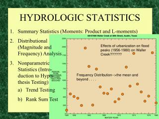
Time series plot • Plot of variable versus time (bar/line/points) • Example. Annual maximum flow series Colorado River near Austin
Interval = 50,000 cfs Interval = 25,000 cfs Interval = 10,000 cfs Histogram • Plots of bars whose height is the number ni, or fraction (ni/N), of data falling into one of several intervals of equal width Dividing the number of occurrences with the total number of points will give Probability Mass Function
Using Excel to plot histograms 1) Make sure Analysis Tookpak is added in Tools. This will add data analysis command in Tools 2) Fill one column with the data, and another with the intervals (eg. for 50 cfs interval, fill 0,50,100,…) 3) Go to ToolsData AnalysisHistogram 4) Organize the plot in a presentable form (change fonts, scale, color, etc.)
Probability density function • Continuous form of probability mass function is probability density function pdf is the first derivative of a cumulative distribution function
Cumulative distribution function • Cumulate the pdf to produce a cdf • Cdf describes the probability that a random variable is less than or equal to specified value of x P (Q ≤ 50000) = 0.8 P (Q ≤ 25000) = 0.4
Flow duration curve • A cumulative frequency curve that shows the percentage of time that specified discharges are equaled or exceeded. • Steps • Arrange flows in chronological order • Find the number of records (N) • Sort the data from highest to lowest • Rank the data (m=1 for the highest value and m=N for the lowest value) • Compute exceedance probability for each value using the following formula • Plot p on x axis and Q (sorted) on y axis
Flow duration curve in Excel Median flow
Statistical analysis • Regression analysis • Mass curve analysis • Flood frequency analysis • Many more which are beyond the scope of this class!
Linear Regression • A technique to determine the relationship between two random variables. • Relationship between discharge and velocity in a stream • Relationship between discharge and water quality constituents A regression model is given by : yi = ith observation of the response (dependent variable) xi = ith observation of the explanatory (independent) variable b0 = intercept b1 = slope ei = random error or residual for the ith observation n = sample size
Least square regression • We have x1, x2, …, xn and y1,y2, …, yn observations of independent and dependent variables, respectively. • Define a linear model for yi, • Fit the model (find b0 and b1) such at the sum of the squares of the vertical deviations is minimum • Minimize Regression applet: http://www.math.csusb.edu/faculty/stanton/m262/regress/regress.html
Linear Regression in Excel • Steps: • Prepare a scatter plot • Fit a trend line Data are for Brazos River near Highbank, TX • Alternatively, one can use ToolsData AnalysisRegression
Coefficient of determination (R2) • It is the proportion of observed y variation that can be explained by the simple linear regression model Total sum of squares, Ybar is the mean of yi Error sum of squares The higher the value of R2, the more successful is the model in explaining y variation. If R2 is small, search for an alternative model (non linear or multiple regression model) that can more effectively explain y variation