Download
1 / 24
240 likes | 247 Views
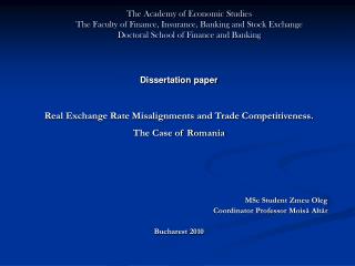
The equilibrium real exchange rate and the Balassa-Samuleson effect in Romania. The Academy of Economic Studies, Doctoral School of Finance and Banking. COORDINATOR, Professor Moisǎ Altǎr. MSc student, Dumitrescu Bogdan Andrei.

E N D
The equilibrium real exchange rate and the Balassa-Samuleson effect in Romania The Academy of Economic Studies, Doctoral School of Finance and Banking COORDINATOR, Professor Moisǎ Altǎr MSc student, Dumitrescu Bogdan Andrei
Dissertation paper outline • The importance of the equilibrium real exchange rate and the Balassa-Samuleson Effect • The aims of the paper • Literature review • The model • The data • Empirical analysis • Concluding remarks • References
The importance of the equilibrium real exchange rate and the Balassa-Samuleson Effect • The equilibrium real exchange rate is very important when judging the external competitiveness of a country. • The equilibrium real exchange rate is also a very important variable for a country who wishes to joinERM II and has to be taken into consideration when setting the central parity. • The Balassa-Samuleson effect has major implications for interpretation of the inflation and the exchange rate criterion for membership in the European Monetary Union
The aims of the paper • To determine the variables that influence the behavior of the equilibrium real exchange rate • To determine the equilibrium value of the real exchange rate using a BEER approach • To determine the misalignment of the real exchange rate from its equilibrium value • To determine the Balassa – Samuleson effect - the extent to which differences in productivity growth between tradable and non-tradable industries explain the observed differences in inflation between Romania and the euro area.
Literature review • The first attempt to determine a countries equilibrium exchange rate was made by Gustav Cassel (1922) who introduced the purchasing power parity. This theory can be seen as a long –term tendency for the exchange rate • Balassa and Samuleson (1964) were the first who showed that the PPP theory is not valid. The existence of non-tradable sector creates important deviations from the level determined by PPP. • Emprical studies that calculated the Balassa- Samuleson effect in Central and eastern Europe: Egert (2003,2004,2005), Candelon and Kool (2006), Oomes (2005),Mihaljek and Klau (2003) • Wiliamson (1994) introduced the concept of fundamental equilibrium exchange rate (FEER) which is the exchange rate consistent with the macroeconomic balance, both internally and externally • Clark and MacDonald (1998) introduced the BEER approach (Behavioral Equilibrium Exchange Rate) which consists in estimating a reduced-form model, that explains the behavior of the real exchange rate on medium and long term. • Emprical studies using BEER in estimating equlibrium exchange rate for CEEC’ Halpern and Wyplosz (2001), De Broeck and Slok (2001), Egert (2002).
The model This paper uses a BEER model in order to estimate equilibrium real exchange rate. The starting point in this model consists in expressing the real exchange rate as a function of the expected value of the real exchange rate at maturity t+k, the real interest rate differential and a time-varying premium-risk: I assume that the unobservable expectation of the exchange rate is determined solely by the long run economic fundamentals The total misalignment from the equilibrium real exchange rate can be expressed: The long-run economic fundamentals used in this paper are:
The Balassa-Samuleson model assumes that real exchange rate is determine by the nominal exchange rate and the relative price differential : We assume Cobb-Douglas production function both in tradable and non-tradable sector: The profit functions can be written : Profit maximisation implies : =0 By log-differentiating the equations above I obtain : The foreign economy (the euro area) is introduced by substituting the above relation into the first equation of the Balassa-Samuleson model:
The data The source of data is Eurostat and The National Bank of Romania database. The economies and periods covered are Romania (1998:1-2006:3) and Euro area (1998:1 - 2006:3). The frequency of observations is quarterly and, in the econometric work, all series are seasonally adjusted using TramoSeats. • Quarterly observations of value added from the production side GDP estimates (decomposed into tradables and non-tradables) • CPI rates of inflation with subcomponents enabling a breakdown into traded and non-traded goods and services • Nominal exchange rates of domestic currency against the euro (quarterly averages) • Employment (quarterly averages) in traded and non-traded industries • Consumption, net foreign assets, openness as a share of GDP. Description of variables: All variables are in constant prices (1998=100) and in the econometric work are expressed in logarithms.
Empirical results In order to estimate the equilibrium real exchange rate using a BEER approach I have followed more steps. First I checked if the series used are stationary : Table 1: Unit root tests for variables included in BEER approach Second I tried to determine a long run relation between variables using cointegration test. First I estimated a VAR. I have chosen the lag length by using Likelihood ratio (LR), Akaike informational criterion (AIC), Schwartz (SIC) şi Hanan-Quinn (HQ)
Table 2 :Choosing the lag length The residual tests performed on the residuals are shown below : Table 3 : Residual tests on VAR
Var also satisfies the stability condition: Table 4 : Checking VAR stability
Next I performed a Johansen cointegration test. First I estimated a vector error correction model : The Johansen rests on examining the rank of the matrix via its eigenvalues. The test showed the presence of two cointegration vectors at both 1% and 5% level.
If we normalize the cointegrating vector with respect to RER, we can obtain the following expression (standard errors in (), t-statistics in [] ) : • An increase in the productivity differential ,in the net foreign assets and in total consumption, will lead to an appreciation of the real exchange rate. • An increase in the degree of openness will cause the current account deficit to widen, which will require real exchange rate depreciation. RER= -1.4336*PROD_DIF - 4.8498*CONS - 0.3151*NFA +1.8390*OPENESS - 0.6816 (0.1545) (0.8637) ( 0.029) (0.1273) [9.2795] [5.6158] [10.6710] [-14.4494] All coefficients are statistically significant and correctly signed.
The next step in the BEER approach requires the estimation of the long run sustainable values for the variables used. In order to do that, I have used a Hodrick-Prescott filter on the extend ARIMA series. Figure 1 : Equilibrium values for total consumption - Hodrick- Prescott filter Figure 2 : Equilibrium value for productivity differential - Hodrick- Prescott filter
Figure 3:Equlilibrium value for net foreign asstes - Hodrick-Prescott filter Figure 4: Equlibrium value for openness - Hodrick-Prescott filter
Figure 5 :The real exchange rate and the real equilibrium exchange rate In order to determine the equilibrium real exchange rate, I have replaced the values obtained by filtering the series in the cointegrating relationship estimated in step 1. : The total misalignment of the real exchange rate from its equilibrium value was obtained by using the next formula : The results are shown below : Figure 6 : Total misalignment real exchange rate from its equilibrium value
Misalignment of the real exchange rates – remarks • During 1998:Q1-2001:Q1 the real exchange rate was undervalued from its equilibrium value, with a maximum misalignment of 28,96% in the first quarter of 1999. This misalignment was caused by the rapid depreciation of the nominal exchange rate induced by the liberalization of prices and of the foreign currency market. Also, the inflations expectations were at a high level which determined the population to keep savings in foreign currency, putting even more pressure on the nominal exchange rate. • During 2001:Q2-2003Q4 the real exchange rate was fairly valued while in 2005Q3-2006Q4 it was slightly undervalued. • In the last period, 2005Q3 -2006Q4, the real exchange rate was overvalued. This situation was caused by the increase in the productivity differential and the appreciation of the nominal exchange rate caused by the large speculative funds attracted by the interest rate differential. The overvaluation can have the effect of losing external competitiveness inducing a larger current account deficit.
Estimation of the Balassa-Samuleson effect The variables used are : the inflation differential between Romania and the euro area, the nominal exchange rate and the productivity differential. The latter is calculated using the next formula : All variables are stationary at the 10% level : Table 6: Unit root tests for variables included in Balassa equation
The estimated equation is : INFL_DIF = 0.7022*L_INFL_DIF(-1) + 0.1822*L_PROD_DIF + 0.2110*L_NOMINAL_ER + 0.1096 (0.0519) (0.0458) (0.0483) (0.0089) All the coefficients are statistically significant and correctly signed. An increase in the nominal exchange rate (which stands for depreciation) and in the productivity differential cause the inflation differential to increase. The linear regression has a high value of R Squared which proves that the inflation differential is well explained by this variables.
I have obtained the Balassa-Samuleson effect by multiplying the coefficient previously determined with the productivity differential. The results are shown below : Table 7 : The Balassa-Samuleson effect in Romania The Balassa-Samuleson effect explained on average only 0.5% of the inflation differential during the covered period. However in the last 2 years the effect was larger because of the increase in the productivity differential. It can be concluded that factors, other than the inflation differential, were responsible for the inflation differential between Romania and the euro area.
Concluding remarks • In the covered period the real exchange rate had some important deviations from its equilibrium value which were determined by the liberalization of the prices and of the foreign exchange market and by the fluctuations of the nominal exchange rate • The nominal exchange rate had a high volatility because of its use by the central bank in order to maintain a low inflation and because of the speculative funds attracted by the interest rate differential. In the last period covered, the real exchange rate seems to be fairly valued which will lead to external competitiveness. • This paper found a negative relation between productivity differential, total consumption, net foreign assets and the real exchange rate which is consistent with the literature. Also, an increase of the degree of openness is likely to cause a depreciation of the real exchange rate because of the increased demand for tradable goods from abroad. • This paper has found evidence of the Balassa-Samuelson effect in Romania • The productivity differential explained on average only 0.5% of the inflation differential in the period covered with a higher impact in 2005 and 2006 (1.17% and 1.31%). The conclusion is that factors different from the productivity differential are responsible for the high inflation differential and that the Balassa-Samuleson effect is not likely to put at risk the Maastricht inflation criterion.
Selected References [1] Balassa, B., (1964), “The purchasing power parity doctrine: A Reappraisal”, Jornal of Political Economy, 6, 584-596 [2] Bergin,P., R. Glick and A.M. Taylor (2006), “Productivity, tradability and the long-run price puzzle”, Journal of Monetary Economics, 53, 2041-2066. [3] De Broek, M. and T. Slok, (2001), ”Interpreting real exchange rate movements in transition countries”, IMF Working Paper 01/56. [4] Brooks, C., (2002), “Introductory econometrics for finance”, Cambridge University Press [5] Candelon,B., K. Raabe, T. van Veen and C. Kool (2006), “Long-run real exchange rate determinants: Evidence from eight new EU member states, 1999-2003”, Journal of comparative economics,35, 87-107. [6] Chudik,A. and J.Mongardini, (2007), “In search of equilibrium: Estimating equilibrium real exchange rates in subsaharan african countries”, IMF Working Paper, 07/90. [7] Clark, P.B.and R. MacDonald, (1998), “Exchange rate and economic fundamentals: A Methodological Comparaison of BEERs and FEERs”, IMF Working Paper 98/67 [8] Coricelli, F.and B Jazbec (2004), “Real exchange rate dynamics in transition economies”, Structural Change and Economic Dynamics, 15, 83-100. [9] Coudert, V. and C. Couharde, (2006), “Real equilibrium exchange rate in European Union New Members and Candidate Countries”, Conference on economic policy issues in the EU, Berlin.
[10] Egert, B.and L. Halpern (2006), ”Equilibrium exchange rates in Central and Eastern Europe: A Meta-Analysis”, Journal of Banking and Finance, 30, 1359-1374. [11] Egert ,B.,(2005), “Equilibrium exchange rates in South EasternEurope, Russia, Ukraine and Turkey: Healthy or (Dutch) diseased?” , Economic Systems, 29, 205-241. [12] Egert, B., I. Drine, K. Lommatzsch and C. Rault, (2003), “The Balassa–Samuelson effect in Central and Eastern Europe: myth or reality?” Journal of Comparative Economics , 31, 552-572. [13] Egert,B., (2002), “Estimating the impact of the Balassa–Samuelsoneffect on inflation and the real exchangerate during the transition”, Economic Systems, 26, 1-16. [14] Faria, J.R. and M. Leon-Ledesma, (2002), “Testing the Balassa–Samuelson effect : Implications for growth and the PPP “,Journal of Macroeconomics, 25, 241-253 [15] Froot, K.A.and K. Rogoff (1994), “Perspectives on PPP and long run real exchange rates”, NBER Working Paper 4952 [16] Klau, M. and D. Mihaljek, (2003), “The Balassa-Samuleson effect in central Europe : a disaggregated analysis”,BIS Working Papers, 143 [17] Lommatzsch, K.and S. Tober, (2005), “What is behind the real appreciation of the accession countries’ currencies?An investigation of the PPI-based real exchange rate”, Economic Systems, 28, 383-403. [18] MacDonald, R., (1997), “What determines real exchange rates? The long and short of it”, IMF Working Paper 97/21