Download
1 / 53
530 likes | 715 Views
Output and the Exchange Rate in the Short Run. Chapter 17 Krugman and Obstfeld 9e ECO41 International Economics Udayan Roy. Long Run and Short Run. Long run theories are useful when all prices of inputs and outputs have enough time to adjust fully to changes in supply and demand.

E N D
Output and the Exchange Rate in the Short Run Chapter 17 Krugman and Obstfeld 9e ECO41 International Economics Udayan Roy
Long Run and Short Run • Long run theories are useful when all prices of inputs and outputs have enough time to adjust fully to changes in supply and demand. • In the short run, some prices of inputs and outputs may not have time to adjust, due to labor contracts, costs of adjustment, or imperfect information about market demand. • This chapter discusses a theory of the short run behavior of a “small” economy with flexible exchange rates under perfect capital mobility
Determinants of Aggregate Demand • Aggregate demand (D) is the aggregate amount of goods and services that people are willing to buy. • It consists of the following types of expenditure: • consumption expenditure (C) • investment expenditure (I) • government purchases (G) • net expenditure by foreigners: the current account (CA)
Determinants of Aggregate Demand • Assumption: Consumption expenditure (C) increases when disposable income (Y− T)—which is income (Y) minus taxes (T)—increases • … but by less than the increase in disposable income • Real interest rates may influence the amount of saving and consumption, but we assume that they are relatively unimportant here. • Wealth may also influence consumption, but we assume that it is relatively unimportant here.
Determinants of Aggregate Demand • Assumption: The balance on the current account (CA) increases … • … when the real exchange rate (q) increases • Recall that the real exchange rate is the price of foreign products relative to the price of domestic products: q = EP*/P • … when disposable income decreases • more disposable income (Y-T) means more expenditure on foreign products (imports). Therefore, when Y−T rises, CA falls.
Current account depends on the real exchange rate and disposable income. Consumption depends on disposable income Investment and government purchases, both exogenous Determinants of Aggregate Demand (cont.) • Aggregate demand is therefore expressed as: • Or more simply: Blue (red) indicates a positive (negative) effect
Aggregate demand as a function of the real exchange rate, disposable income, investment, government purchases Value of output, income, and expenditure Short Run Equilibrium for Aggregate Demand and Output • Equilibrium is achieved in the goods market when output equals aggregate demand: Y = D. • or
Goods Market Equilibrium • Note that only Y and E are endogenous (or, unknown) variables in this equation • The others—T, I, G, P, and P*—are exogenous constants in our short-run analysis • So, what does the goods market equilibrium equation tell us about how Y and E are related?
Goods Market Equilibrium • If Y increases by, say, $100, then C will increase too, but by less. Let’s say C increases by $70 • Then to maintain equilibrium, CAmust increase (in this case, by $30) • But the increase in Y, by itself, reducesCA • So, the increase in Y must be accompanied by an increase in E • (so that CA can increase, as necessary)
Goods Market Equilibrium: DD Curve • For given values of the exogenous variables—T, I, G, P, and P*—the endogenous unknowns, Y and E, must move in the same direction
Goods Market Equilibrium: Shifts of the DD Curve Suppose the economy is initially at Point 1. Suppose there is a tax hike (T↑), but output is still at Y1. Then, C will decrease. Let’s say C decreases by $100. This will require CA to increase by $100. But T ↑, by itself, will increase CAby less than $100. DD2 Why? When C falls by $100, the consumption of imported goods would fall by less: say, by $55. So, the tax cut, by itself, would increase CA by only $55. 3 Therefore, to make CA increase by another $45, E must increase. So, the tax hike takes the economy from Point 1 to Point 3. In other words, a tax increase shifts the DD curve upward and to the left.
Goods Market Equilibrium: Shifts of the DD Curve Suppose the economy is initially at Point 2. Suppose I or G increases (I + G↑), but output is still at Y2. Then, CA must decrease. With unchanged Y, this requires a decrease in E. Therefore, if I or G increases and Y is unchanged, then the economy must move from Point 2 to Point 3. In other words, if I or Gincreases, the DD curve must shift downward or to the right. DD2 3
Goods Market Equilibrium: Shifts of the DD Curve Suppose the economy is initially at Point 2. Suppose P* increases or P decreases (P*/P↑), but output is still at Y2. Then, CA must stay unchanged. With Y and T unchanged, the only way CA can remain unchanged in spite of P*/P↑ is if E decreases enough to keep the real exchange rate unchanged. Therefore, if P* increases or P decreases and Y is unchanged, then the economy must move from Point 2 to Point 3. In other words, if P* increases or P decreases , the DD curve must shift downward or to the right. DD2 3
Shifting the DD Curve • The DD curve shifts right if: • G increases • T decreases • I increases • P decreases • P* increases • C increases for some unknown reason • CA increases for some unknown reason Y = D(E×P*/P, Y – T, I, G)
Short Run Equilibrium for Assets • We consider two asset markets when considering asset market equilibrium: • Ch 14: Foreign exchange market • interest parity: R = R* + (Ee – E)/E • Ch 15: Money market • real money supply and demand determine equilibrium: Ms/P = L(R, Y)
Equilibrium in Asset Markets • Let us simplify the money market equilibrium equation to or equivalently to • The interest parity equation then yields • This is the equation for the AA curve
Equilibrium in Asset Markets • Suppose the economy is initially at Point 2 • Suppose there is a decrease in Ms or R* or Ee, or an increase in L0 or P • If E stays unchanged at E2, then Y must decrease • The economy must go from Point 2 to, perhaps, Point 3 • In other words, a decrease in Ms or R* or Ee, or an increase in L0 or P shifts the AA curve left 3 AA2
Shifting the AA Curve • The AA curve shifts right if: • Ms increases • P decreases • Ee rises • R* rises • L decreases for some unknown reason E E0 E1 Y Y0 Y1
Putting the Pieces Together: the DD and AA Curves • A short run equilibrium means that the exchange rate (E) and output (Y) are such that there is equilibrium in: • the output market: aggregate demand (D) equals aggregate output (Y). • the foreign exchange market: interest parity holds. • the money market: real money supply (MS/P) equals real money demand (L). Y = D(E×P*/P, Y – T, I, G)
Fig. 17-8: Short-Run Equilibrium: The Intersection of DD and AA The short run equilibrium occurs at the intersection of the DD and AA curves The output market is in equilibrium on the DD curve The assetmarkets are in equilibrium on the AA curve
Shifting the AA and DD Curves • The AA curve shifts right if: • Ms increases • P decreases • Ee rises • R* rises • L decreases for some unknown reason • The DD curve shifts right if: • G increases • T decreases • I increases • P decreases • P* increases • C increases for some unknown reason • CA increases for some unknown reason Knowing how some specified change shifts the DD and AA curves will help us predict the consequences of the specified change.
Temporary Changes in Monetary and Fiscal Policy • Monetary policy: policy in which the central bank influences the money supply (MS). • Monetary policy primarily influences asset markets. • Fiscal policy: policy in which governments influence the amount of government purchases (G) and taxes (T). • Fiscal policy primarily influences aggregate demand (D). • Temporary policy changes are expected to be reversed in the near future and thus do not affect expectations about exchange rates in the long run. • Specifically, temporary changes in MS, G, and T do not affect Ee.
Shifting the AA and DD Curves • The AA curve shifts right if: • Ms increases • P decreases • Ee rises • R* rises • L decreases for some unknown reason (L0↓) • The DD curve shifts right if: • G increases • T decreases • I increases • P decreases • P* increases • C increases for some unknown reason • CA increases for some unknown reason
Temporary Changes in Monetary Policy • When there is an increase in the supply of money • The AA shifts up (right) and DD is unaffected. • Both E and Y increase • R decreases • As Ee is unaffected when the change in Ms is temporary, the increase in E leads to a decrease in R; recall R = R* + (Ee/E) – 1. E DD E0 Y Y0
Fig. 17-10: Effects of a Temporary Increase in the Money Supply R*↑ and Ee↑ have the same effect, as does a fall in money demand (L).
Effect of Temporary MS↑ on CA • There are two ways to figure out the effect of a change in an exogenous variable on a country’s current account • Recall that in goods market equilibrium • Method 1: • Method 2: We will return to Ch. 16 and use this to analyze the long-run behavior of CA.
Effect of Temporary MS↑ on CA • Method 2: • An increase in Ms causes Y to increase. • But C(Y – T) increases less than Y does. • Therefore, CA must increase. • That is, an increase in the supply of money, leads to an increase in the current account balance (or, net exports) R*↑ and Ee↑ have the same effect, as does a fall in money demand (L).
Changes in Ee and R* • Any increase in Ee, the expected future value of the foreign currency, or in R*, the foreign interest rate cause the same shifts as expansionary monetary policy: they shift the AA curve rightward and do not affect the DD curve • Therefore, Y↑ and E↑. • As P and P*, being exogenous, are unaffected, E↑ implies q↑
Changes in Ee and R* • Recall that the money market’s equilibrium equation is or, equivalently, • As L0, P, and Ms, being exogenous, are unaffected by increases in Eeor R*, the fact that Y↑ implies R↑
Changes in Ee and R* • Recall that • We have just seen that Ee↑ or R*↑ causes Y↑ • When Y↑ and T is unchanged, C increases but by less. • Therefore, Y− C↑ • As I and G are exogenous and, therefore, unaffected by changes in Eeor R*, it must be that CA↑
Temporary Changes in Fiscal Policy • An increase in government purchases or a decrease in taxes increases aggregate demand and output. • The DD curve shifts right. • Higher output increases real money demand, and • thereby increases interest rates, • causing an increase in the value of the domestic currency (a fall in E).
Shifting the AA and DD Curves • The AA curve shifts right if: • Ms increases • P decreases • Ee rises • R* rises • L decreases for some unknown reason • The DD curve shifts right if: • G increases • T decreases • I increases • P decreases • P* increases • C increases for some unknown reason • CA increases for some unknown reason
Fig. 17-11: Effects of a Temporary Fiscal Expansion G↑ and/or T ↓ P*↑and I↑ have the same effect, as do shocks that increase C and CA. E↓implies R↑ because R = R* +(Ee/E) – 1.
Effect of G↑ and/or T↓ on CA • When G↑ and/or T↓ — this is called expansionary fiscal policy — E↓ and Y↑. • Therefore, CA↓. • Expansionary (contractionary) fiscal policy reduces (increases) net exports.
Fig. 17-12: Maintaining Full Employment After a Temporary Fall in World Demand for Domestic Products Temporary fall in world demand for domestic products reduces output below its normal level Temporary monetary expansion could depreciate the domestic currency Temporary fiscal policy could reverse the fall in aggregate demand and output
Fig. 17-13: Policies to Maintain Full Employment After a Money Demand Increase Temporary monetary policy could increase money supply to match money demand Increase in money demand raises interest rates and appreciates the domestic currency Temporary fiscal policy could increase aggregate demand and output
Effects of an increase in investment • Simply put, the effects of I↑ are exactly the same as those of G↑ • Therefore, we can predict that if G↑ and/or I↑, then E↓, q↓, Y↑, R↑, and CA↓.
Effects of a change in foreign prices • We saw three slides back that P*↑ causes the DD curve to shift right and has no effect on the AA curve • Therefore, E↓ and Y↑. • And, following the same steps as in our discussion of the effects of Ee↑ and R*↑, we can prove that CA↑
Shifting the AA and DD Curves • The AA curve shifts right if: • Ms increases • P decreases • Ee rises • R* rises • L decreases for some unknown reason • The DD curve shifts right if: • G increases • T decreases • I increases • P decreases • P* increases • C increases for some unknown reason • CA increases for some unknown reason
Effects of a change in domestic prices • Recall that P↓ causes both AA and DD curves to shift rightward • Therefore, Y↑ is certain • But E could decrease, stay unchanged, or increase, as in the three diagrams below E E E DD DD DD AA AA AA Y Y Y
Effects of a change in domestic prices • Following the same steps as in our discussion of the effects of Ee↑ and R*↑ and P*↑, we can prove that CA↑ • Finally, the interest parity equation () implies that, as Eeand R* are exogenous and, therefore, unaffected by P↓, the ambiguous behavior of E implies R too could decrease, stay unchanged, or increase
Summary: Short Run Predictions, Flexible Exchange Rate System The predictions above are for temporary changes in the exogenous variables. The exogenous variables—policy variables and ‘shocks’—are listed on the first column and the endogenous unknowns are listed on the first row. The 2nd and 3rd columns show how the DD and AA curves are shifted by an increase in the exogenous variables.
Permanent Changes in Monetary and Fiscal Policy • Permanent policy changes modify people’s expectations about future exchange rates (Ee) … • … when they change the long-run value of E.
Permanent Increase in Money Supply • The AA curve shifts right because of the increase in MS. The equilibrium moves from point 1 to point 3 in Fig 17-14. • In the long run, E will rise. See Table 16-1. • This will have the immediate effect of raising Ee. • The increase in Ee shifts the AA curve to the right again. • The equilibrium moves from point 3 to point 2 in Fig 17-14. • Both E and Y increase more for a permanent increase in MS than for a temporary increase in MS.