Download
1 / 14
140 likes | 274 Views
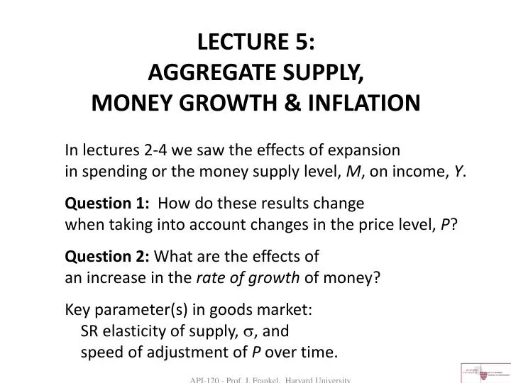
LECTURE 5: AGGREGATE SUPPLY, MONEY GROWTH & INFLATION. In lectures 2-4 we saw the effects of expansion in spending or the money supply level, M , on income, Y . Question 1: How do these results change when taking into account changes in the price level, P ?

E N D
LECTURE 5: AGGREGATE SUPPLY, MONEY GROWTH & INFLATION • In lectures 2-4 we saw the effects of expansion in spending or the money supply level, M, on income, Y. • Question 1: How do these results change when taking into account changes in the price level, P? • Question 2: What are the effects of an increase in the rate of growth of money? • Key parameter(s) in goods market: SR elasticity of supply, , and speed of adjustment of P over time. API-120 - Prof. J. Frankel, Harvard University
AGGREGATE DEMAND • Everything we have learned so far, about the effects of demand expansion, including monetary & fiscal policy, now goes into the AD relationship, but holds only for a give price level P. • The Aggregate Demand curve allows the price level to vary. API-120 - Prof. J. Frankel, Harvard University
Aggregate Demand Curve Slope of AD: p P↑ => => LM shifts left => Y . Spending increase Ā↑ shifts AD right (by multiplier, less crowding out). Money increase M↑ shifts AD up (in direction proportion to M). negative AD y Shift of AD p AD' AD y API-120 - Prof. J. Frankel, Harvard University
p p y y OVERVIEW OF AGGREGATE SUPPLY • Ultra-Keynesian case:AS flat, at => AD expansion goes entirely into Y. AD' AS Realistic in Very Short Run. • Classical caseAS vertical at => AD expansion goes entirely into P. AS AD' Realistic in Long Run. API-120 - Prof. J. Frankel, Harvard University
OVERVIEW OF AGGREGATE SUPPLY (continued) ● Robert Lucas Milton Friedman API-120 - Prof. J. Frankel, Harvard University
Monetary expansion raises AD in the SR • An increase in the current level of M shifts LMcurve out (because M/P in the SR). • An increase in the expected future rate of growthof M shifts IS out, because e=> r=> A .(See next slide). • Either way, IS-LM shifts right=> AD shifts right: => Y↑ for given P => AD shifts right. API-120 - Prof. J. Frankel, Harvard University
The real interest rate & the cost of capital Business investment, & other components of spending A, depend not just on the nominal interest rate i, but on the real interest rate r ≡ i - e . (To compute corporate cost of capital, it should also be long-term i, and adjusted for taxes.) This becomes important when we allow for steady-state rate of change in M & P, i.e., inflation. Generally, e is not fully reflected in i in SR. So => r => A => IS shifts right => “Mundell effect.” API-120 - Prof. J. Frankel
STANLEY FISCHER (MIT PRESS, 2004) • Over time, P rises in response to high AD& Y. • In LR, P rises in same proportionas M. • ≡ “Neutrality of money.” API-120 - Prof. J. Frankel, Harvard University
SUMMARY OF EFFECTS OF 2 EXPERIMENTS i by same as πe (Fisher effect) => M/P. API-120 - Prof. J. Frankel, Harvard University
Intellectual History of the Increasing Ineffectivenessof Monetary Policy at Stabilizing Output Monetary expansion can raise Y? A.S. -- at the cost of higher P. Phillips curve (1958) -- at the cost of higher inflation, . Friedman & Phelps(1968) at the cost of ever-acceleratingNatural Rate Hypothesis. -- (because πe adjusts over time to π). Lucas, Sargent, Barro (1972-78) only randomly Rational Expectations -- (because π-πe must be random). Kydland-Prescott (1977) & Barro- and, worse yet: monetary discretionGordon(1983). Time-inconsistency-- => inflationary bias. E.g., Bruno-Easterly(1998) & High (>40%)hurts growth Dornbusch-Fischer (1993) -- in the LR. (Chart 1) (Table 2) API-120 - Prof. J. Frankel, Harvard University
Inflation above a threshold ≈ 40% tends to have a negative effect on growth. Source: API-120 - Prof. J. Frankel, Harvard University
An example of predictable inflation: The Mexican sexenio From 1976 through 1994, inflation would shoot up every 6th year (presidential election years). 1982 1988 1994 1976 and the peso would devalue, API-120 - Prof. J. Frankel, Harvard University
The Mexican sexenio, continuedExample of rational expectations: investors came to anticipate inflation & devaluation after elections, and so would pull out ahead of time. 1982 1988 1994 J.Bianchi, J.C.Hatchondo, L.Martinez, 2013, “International Reserves and Rollover Risk,” FRB Richmond WP13-01R , NBER WP 18628 API-120 - Prof. J. Frankel, Harvard University
Addendum:What lessons will monetary theory takefrom the 2008 global financial crisis? • One is that excessive monetary ease can show up in the form of asset price “bubbles” • which can lead to crashes & recessions, • and not necessarily always in the form of inflation • which can lead to crashes & recessions. API-120 - Prof. J. Frankel, Harvard University