Download
1 / 22
220 likes | 391 Views
B.5.2 - Concavities and the Second Derivative Test. Calculus - Santowski. Lesson Objectives. 1. Calculate second and third derivatives of functions 2. Define concavity and inflection point 3. Test for concavity in a function using the second derivative

E N D
B.5.2 - Concavities and the Second Derivative Test Calculus - Santowski Calculus - Santowski
Lesson Objectives • 1. Calculate second and third derivatives of functions • 2. Define concavity and inflection point • 3. Test for concavity in a function using the second derivative • 4. Perform the second derivative test to determine the nature of relative extrema • 5. Apply concepts of concavity, second derivatives, inflection points to a real world problem Calculus - Santowski
Fast Five • 1. Solve f’’(x) = 0 if f(x) = 3x3 - 4x2 + 5 • 2. Find the x co-ordinates of the extrema of f(x) = 2x - lnx • 3. Sketch a graph of a function that has an undefined derivative at x = c which (i) does and (ii) does not change concavities. • 4. Find the 4th derivative of f(x) = x4 + 2x3 + 3x2 - 5x + 7 • 5. If the position, as a function of time, of a vehicle is defined by s(t) = t3 - 2t2 - 7t + 9, find acceleration at t = 2 Calculus - Santowski
(B) New Term – Graphs Showing Concavity Calculus - Santowski
Concavity is best “defined” with graphs (i) “concave up” means in simple terms that the “direction of opening” is upward or the curve is “cupped upward” An alternative way to describe it is to visualize where you would draw the tangent lines you would have to draw the tangent lines “underneath” the curve (B) New Term – Concave Up Calculus - Santowski
Concavity is best “defined” with graphs (ii) “concave down” means in simple terms that the “direction of opening” is downward or the curve is “cupped downward” An alternative way to describe it is to visualize where you would draw the tangent lines you would have to draw the tangent lines “above” the curve (B) New Term – Concave down Calculus - Santowski
(B) New Term – Concavity • In keeping with the idea of concavity and the drawn tangent lines, if a curve is concave up and we were to draw a number of tangent lines and determine their slopes, we would see that the values of the tangent slopes increases (become more positive) as our x-value at which we drew the tangent slopes increase • This idea of the “increase of the tangent slope is illustrated on the next slides: Calculus - Santowski
(B) New Term – Concavity Calculus - Santowski
(B) New Term – Inflection Point • An inflection point is the point on a function where the function changes its concavity (see the black points on the red curve) • Mathematically, inflection points are found where y’’(x) = 0 • Inflection points can also be found where y’’(x) is undefined Calculus - Santowski
Consider the graphs of the following functions and determine: (i) y’’(x) (ii) where the inflection points are (iii) what their intervals of concavity are F(x) = (x - 1)4 G(x) = x^(1/5) H(x) = x^(2/3) I(x) = 1/x (B) New Terms - Concavity and Inflection Points Calculus - Santowski
(B) New Terms - Concavity and Inflection Points Calculus - Santowski
(C) Functions and Their Derivatives • In order to “see” the connection between a graph of a function and the graph of its derivative, we will use graphing technology to generate graphs of functions and simultaneously generate a graph of its derivative • Then we will connect concepts like max/min, increase/decrease, concavities on the original function to what we see on the graph of its derivative Calculus - Santowski
(C) Functions and Their Derivatives Calculus - Santowski
Points to note: (1) the fcn has a minimum at x=2 and the derivative has an x-intercept at x=2 (2) the fcn decreases on (-∞,2) and the derivative has negative values on (-∞,2) (3) the fcn increases on (2,+∞) and the derivative has positive values on (2,+∞) (4) the fcn changes from decrease to increase at the min while the derivative values change from negative to positive (5) the function is concave up and the derivative fcn is an increasing fcn (6) the second derivative graph is positive on the entire domain (C) Functions and Their Derivatives Calculus - Santowski
(C) Functions and Their Derivatives Calculus - Santowski
f(x) has a max. at x = -3.1 and f `(x) has an x-intercept at x = -3.1 f(x) has a min. at x = -0.2 and f `(x) has a root at –0.2 f(x) increases on (-∞, -3.1) & (-0.2,∞) and on the same intervals, f `(x) has positive values f(x) decreases on (-3.1, -0.2) and on the same interval, f `(x) has negative values At the max (x = -3.1), the fcn changes from being an increasing fcn to a decreasing fcn è the derivative changes from positive values to negative values At a the min (x = -0.2), the fcn changes from decreasing to increasing -> the derivative changes from negative to positive f(x) is concave down on (-∞, -1.67) while f `(x) decreases on (-∞, -1.67) and the 2nd derivative is negative on (-∞, -1.67) f(x) is concave up on (-1.67, ∞ ) while f `(x) increases on (-1.67, ∞) and the 2nd derivative is positive on (-1.67, ∞) The concavity of f(x) changes from CD to CU at x = -1.67, while the derivative has a min. at x = -1.67 (C) Functions and Their Derivatives Calculus - Santowski
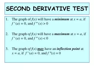
(C) Functions and Their Derivatives - Summary • If f ``(x) >0, then f(x) is concave up • If f `(x) < 0, then f(x) is concave down • If f ``(x) = 0, then f(x) is neither concave nor concave down, but has an inflection points where the concavity is then changing directions • The second derivative also gives information about the “extreme points” or “critical points” or max/mins on the original function: • If f `(x) = 0 and f ``(x) > 0, then the critical point is a minimum point (picture y = x2 at x = 0) • If f `(x) = 0 and f ``(x) < 0, then the critical point is a maximum point (picture y = -x2 at x = 0) • These last two points form the basis of the “Second Derivative Test” which allows us to test for maximum and minimum values Calculus - Santowski
(D) Examples - Algebraically • Find where the curve y = x3 - 3x2 - 9x - 5 is concave up and concave down. Find and classify all extreme points. Then use this info to sketch the curve. • f(x) = x3 – 3x2 - 9x – 5 • f `(x) = 3x2 – 6x - 9 = 3(x2 – 2x – 3) = 3(x – 3)(x + 1) • So f(x) has critical points (or local/global extrema) at x = -1 and x = 3 • f ``(x) = 6x – 6 = 6(x – 1) • So at x = 1, f ``(x) = 0 and we have a change of concavity • Then f ``(-1) = -12 the curve is concave down, so at x = -1 the fcn has a maximum point • Also f `(3) = +12 the curve is concave up, so at x = 3 the fcn has a minimum point • Then f(3) = -33, f(-1) = 0 as the ordered pairs for the function Calculus - Santowski
(D) In Class Examples • ex 1. Find and classify all local extrema using FDT of f(x) = 3x5 - 25x3 + 60x. Sketch the curve • ex 2. Find and classify all local extrema using SDT of f(x) = 3x4 - 16x3 + 18x2 + 2. Sketch the curve • ex 3. Find where the curve y = x3 - 3x2 is concave up and concave down. Then use this info to sketch the curve • ex 4. For the function find (a) intervals of increase and decrease, (b) local max/min (c) intervals of concavity, (d) inflection point, (e) sketch the graph Calculus - Santowski
(D) In Class Examples • ex 5. For the function f(x) = xex find (a) intervals of increase and decrease, (b) local max/min (c) intervals of concavity, (d) inflection point, (e) sketch the graph • ex 6. For the function f(x) = 2sin(x) + sin2(x), find (a) intervals of increase and decrease, (b) local max/min (c) intervals of concavity, (d) inflection point, (e) sketch the graph • ex 7. For the function , find (a) intervals of increase and decrease, (b) local max/min (c) intervals of concavity, (d) inflection point, (e) sketch the graph Calculus - Santowski
(I) Internet Links • We will work on the following problems in class: Graphing Using First and Second Derivatives from UC Davis • Visual Calculus - Graphs and Derivatives from UTK • Calculus I (Math 2413) - Applications of Derivatives - The Shape of a Graph, Part II Using the Second Derivative - from Paul Dawkins • http://www.geocities.com/CapeCanaveral/Launchpad/2426/page203.html Calculus - Santowski
(J) Homework • Textbook, p307-310, • (i) Graphs: Q27-32 • (ii) Algebra: higher derivatives; Q17,21,23 • (iii) Algebra: max/min; Q33-44 as needed + variety • (iv) Algebra: SDT; Q50,51 • (v) Word Problems: Q69,70,73 • photocopy from Stewart, 1997, Calculus – Concepts and Contexts, p292, Q1-26 Calculus - Santowski