Download

1 / 34
340 likes | 460 Views
Multivariate Response: Changes in G. Overview. Changes in G from disequilibrium (generalized Bulmer Equation) Fragility of covariances to allele frequency change Resource-partitioning models and genetic correlations Long-term directional selection: drift

E N D
Overview • Changes in G from disequilibrium (generalized Bulmer Equation) • Fragility of covariances to allele frequency change • Resource-partitioning models and genetic correlations • Long-term directional selection: drift • Long-term directional selection: mutation • Long-term quadratic (stabilizing) selection
Infinitesimal Model: Changes in G from linkage disequilibrium The “Bulmer effect” --- changes in variances from LD produced by selection also applies to covariances Hence, G(t) = G(0) + D(t), where D is a matrix of all pairwise disequilibrium contributions Dynamics of D as with univariate case: half the value removed by recombination (unlinked)
If dt is the current LD and dt* is the LD generated by selection of the parents, then the LD in offspring changes by The LD generated by selection is just Gt*-Gt, where G* is the G matrix after selection (but before reproduction)
Where phenotypes and breeding values are multivariate-normally distributed, then the within-generation change in G is a function of the within-generation change in P, Putting these together gives the multivariate version of the Bulmer equation (due to Tallias) as
Change in the genetic variance Any change in the mean reduces the variance Note that the can be no direct selection on i (bi = 0), but if we have a response, get reduction in variance Now consider changes in covariances Directional selection in same direction = reduction in covariance Directional selection in different directions = increase in covariance Sign of gij determines effect of quadratic selection on covariance
Asymmetric responses can occur Under the standard breeder’s equation, the correlated response is CR1 =S2 h2 h1 rA, so CR1 = CR2 , so long as S1 = S2 This is no longer true under the infinitesimal model, as the covariances change and which trait (1 or 2) is selected differentially changes the covariance. When disequilibrium-driven selection asymmetries occur, the correlated response will be smaller when selecting on the trait with the higher heritability, as this produces the largest reduction of the genetic covariance.
A very common fitness function is the Gaussian The Bulmer equation has a simple form when using this fitness function, Changes in G under Gaussian fitness functions If phenotypes and BVs are multivariate normal before selection, they remain so afterwards
Allele frequency change Two sources generating genetic covariances Linkage disequilibrium: alleles with effects on only single traits can become associated, creating a covariance Pleiotropy: an allele influences two (or more) traits Changes in G from linkage are transient, as the association decays away once selection stops Changes in G from pleiotropy are permanent, as the allele frequencies do not change once selection stops
Changes in covariance when allele frequency change occurs Recall that the heritability provides very little information as to how the variance changes when allele frequencies change Genetic covariances are more fragile than genetic variances Smaller allele frequency change can have larger effects than changes on variance Hidden pleiotropy: Lots of pleiotropic alleles present but there effects cancel, so no net covariance.
complementary pleiotropy: ++ or -- antagonistic pleiotropy: +- or -+ Hidden Pleiotropy: roughly equal numbers of each, no NET genetic correlation In this case, allele frequency change can produce either a positive or negative genetic correlation Thus, a pair of traits with no initial genetic correlation could, in the extreme, either consist of all no pleiotropic alleles or all pleiotropic alleles. Very different outcomes result from these two states
Models of covariance changes under allele frequency change Hazel, Lush, and Lerner proposed that selection to move two traits in the same direction increases the relative frequency of antagonistic pleiotropic alleles, making genetic covariances more negative as selection proceeds. ++ and -- alleles are quickly lost (or fixed) by selection, while -+ and +- alleles experience less selective pressure, and therefore experience slower allele frequency change Some experimental support for this: Friars et al. 1962: Genetic correlations measured from 1949 to 1957 in a series of chicken lines for production traits. 16 of the 18 correlations showed a negative trend
Genetic Covariances are More Fragile Than Genetic Variances Classic paper of Bohren, Hill, Robertson (1966) Theoretical results and simulations showed covariances change more quickly, and more erratically, than variances. Confirmed the general suggestion by Hazel et al than eventually genetic covariances generally become more negative. However, depending on the distribution of allele frequencies and effects,that the genetic covariance may actually increase in the first few generations
Can Antagonistic Pleiotropy Maintain Variation? Several workers suggested that alleles having antagonistic pleiotropic effects on different life-history fitness components (such as reducing fecundity while increasing life span) might be maintained in the population Same logic, but different outcome from Hazel et al suggestion, which was that such alleles would have longer persistance times, but did not cover if they would be maintained by selection Curtsinger et al. Model for this:
Range of parameters allowing for polymorphism is quite narrow, esp. for weak selection. As detailed in the notes, this model likely overestimates the chance of maintaining polymorphisms.
Nature of Pleiotropic covariances What makes a pleiotropic effect antagonistic vs. complementary? Resource-partitioning models offer some insight Alleles contributing to the acquisition of the common resource R are complementary Alleles contributing to the allocation of this common are antagonistic Obviously, the relative frequencies of these classes of alleles (and their variances) determine if a covariance is positive or negative
Key: Tradeoffs (allocation of the common resource) do no automatically mean negative genetic covariances!
Long term directional selection response: Drift The simplest model to accommodate allele frequency changes is the infinitesimal with drift. When all genetic variance is additive, the expected value of G has a simple form: Hence, the expected cumulative response after t generations is just
If we assume a constant amount of directional selection each generation, the cumulative response simplifies to The expected total response from the genetic variation initially present thus becomes This is the multivariate form of Robertson’s limit: total response is 2Ne * inital response Tradeoff: as stronger selection gives initially larger response but smaller Ne, and hence smaller total response
If M denotes the matrix of mutational input, then the mutation-drift equilibrium is Long term directional selection response: drift and new mutation Keeping within the infinitesimal framework, now lets consider the joint effects of drift removing variation, mutation adding it. The G matrix at time t thus becomes
Putting these together, the cumulative response by generation t becomes We can decompose this two ways. First, the asymptotic response plus the response from the residual component due to the initial variation
Alternatively, we can decompose the total response into the response from the original variation and the response from new mutation, For any particular trait, the ratio of component 2 to the total response is the fraction of response due to new mutation (variation not present at the start of selection).
Long term response: Balance between directional and stabilizing selection (infinitesimal model results) One class of models for a selection limit is the balance between directional (which could be artificial) and stabilizing selection. Zeng looked at this problem using a generalized Gaussian fitness function The matrix W describes the nature of quadratic (stabilizing) selection, while the difference between the population mean m and the optimal value y describes the directional selection component
Under this model, the within-generation change in the vector of means and the phenotypic covariance matrix are Previous results describe the change in G, while the change in mean is Zeng’s key observation was that when the change in mean equals zero, the solution is independent of the genetic covariance structure G
Long term response: Critically depend on the distribution of allelic effects The infinitesimal-based models avoid the need to consider the messy genetic details. In reality, they are important. Model for artificial selection: The traits of interest were in a mutation-(natural) selection balance, and this the variation that forms the foundation for the initial response. Two general classes of approximations used in mutation-selection models: Gaussian genetic models and House-of-cards (HOC) models
Gaussian genetic model Effects of selection relative to mutation are weak, many alleles at a locus, distribution of effects roughly normal. House-of-Cards model Effects of selection relative to mutation are strong, few alleles at a locus, most rare. Highly leptokurtic distribution of allele frequencies, with rare alleles having significant effects
Which model is assumed makes a major difference for long-term response, as simulations by Reeve showed:
Long term response: Balance between directional and stabilizing selection (finite-locus model results) Key result: If pleiotropic alleles are present, they can have a significant impact on the dynamics of the change in even, even if there is no genetic covariance between traits. Baatz and Wagner considered a two-trait model with directional selection on one trait and stabilizing on the other. The change in mean turns out to be a function of s(g1,g22), which can be nonzero, even when there is no correlation among breeding values, s(g1,g2), =0. This can easily happen with hidden pleiotropy. Consider a favorable rare allele that increases trait 1 and also have an impact on trait 2 (positively or negatively)
Baatz and Wagner call this the Pooh effect, after Winnie the Pooh eating to much honey and getting stuck in rabbit’s house As directional selection tries to drive this allele to a higher frequency, it also increases the variance at trait 2, increasing the strength of selection against in. In the extreme, this later selection an be sufficiently strong as to stop directional selection
Long term response: Stabilizing selection Mutation-selection balance Much work has been done on mutation-selection balance problems with stabilizing selection on a trait (or traits) removing selection while mutation introduces it. Problem: The models don’t work: Selection in the wild is too strong to account for the high levels of genetic variation seen Classic analysis: Kimura-Lande model assuming Gaussian distribution of allelic effects at each locus
Under gaussian stabilizing selection, we have The equilibrium G matrix is the sum over all loci, If there is no net pleiotropy, we have
Common orientation of g and G?? Are the axes of G and the quadratic fitness surface similar? I.e., can G evolve to have axes similar to g? Hunt et al. (Example 31.5). Male call components in the cricket Teleogryllus commodus
Model Assumptions, Genetic Correlations, and Hidden Pleiotropy