Download
1 / 153
1.54k likes | 1.71k Views
Adaptive annealing: a near-optimal connection between sampling and counting. Daniel Štefankovič (University of Rochester) Santosh Vempala Eric Vigoda (Georgia Tech). Adaptive annealing: a near-optimal connection between sampling and counting. If you want to count

E N D
Adaptive annealing: a near-optimal connectionbetween sampling and counting Daniel Štefankovič (University of Rochester) Santosh Vempala Eric Vigoda (Georgia Tech)
Adaptive annealing: a near-optimal connectionbetween sampling and counting If you want to count using MCMC then statistical physics is useful. Daniel Štefankovič (University of Rochester) Santosh Vempala Eric Vigoda (Georgia Tech)
Outline 1. Counting problems 2. Basic tools: Chernoff, Chebyshev 3. Dealing with large quantities (the product method) 4. Statistical physics 5. Cooling schedules (our work) 6. More…
Counting independent sets spanning trees matchings perfect matchings k-colorings
Counting independent sets spanning trees matchings perfect matchings k-colorings
Compute the number of spanning trees
Compute the number of spanning trees det(D – A)vv Kirchhoff’s Matrix Tree Theorem: - det D A
Compute the number of spanning trees polynomial-time algorithm G number of spanning trees of G
? Counting independent sets spanning trees matchings perfect matchings k-colorings
Compute the number of independent set subset S of vertices, of a graph no two in S are neighbors = independent sets (hard-core gas model)
# independent sets = 7 independent set = subset S of vertices no two in S are neighbors
# independent sets = G1 G2 G3 ... Gn-2 ... Gn-1 ... Gn
# independent sets = 2 G1 3 G2 5 G3 ... Gn-2 Fn-1 ... Gn-1 Fn ... Gn Fn+1
# independent sets = 5598861 independent set = subset S of vertices no two in S are neighbors
Compute the number of independent sets ? polynomial-time algorithm G number of independent sets of G
Compute the number of independent sets (unlikely) ! polynomial-time algorithm G number of independent sets of G
graph G # independent sets in G #P NP FP P #P-complete #P-complete even for 3-regular graphs (Dyer, Greenhill, 1997)
graph G # independent sets in G ? approximation randomization
graph G # independent sets in G ? which is more important? approximation randomization
graph G # independent sets in G My world-view: (true) randomness is important conceptually but NOT computationally (i.e., I believe P=BPP). approximation makes problems easier (i.e., I believe #P=BPP) ? which is more important? approximation randomization
We would like to know Q Goal: random variable Y such that P( (1-)Q Y (1+)Q ) 1- “Y gives (1)-estimate”
We would like to know Q Goal: random variable Y such that P( (1-)Q Y (1+)Q ) 1- (fully polynomial randomized approximation scheme): FPRAS: Y polynomial-time algorithm G,,
Outline 1. Counting problems 2. Basic tools: Chernoff, Chebyshev 3. Dealing with large quantities (the product method) 4. Statistical physics 5. Cooling schedules (our work) 6. More...
We would like to know Q X1 + X2 + ... + Xn Y= n 1. Get an unbiased estimator X, i. e., E[X] = Q 2. “Boost the quality” of X:
The Bienaymé-Chebyshev inequality P( Y gives (1)-estimate ) 1 V[Y] 1 - E[Y]2 2
The Bienaymé-Chebyshev inequality P( Y gives (1)-estimate ) 1 V[Y] 1 - E[Y]2 2 squared coefficient of variation SCV X1 + X2 + ... + Xn V[Y] V[X] 1 Y= = n E[Y]2 E[X]2 n
The Bienaymé-Chebyshev inequality X1 + X2 + ... + Xn Y= n Let X1,...,Xn,X be independent, identically distributed random variables, Q=E[X]. Let Then P( Y gives (1)-estimate of Q ) 1 V[X] 1 - 2 n E[X]2
Chernoff’s bound X1 + X2 + ... + Xn Y= n Let X1,...,Xn,X be independent, identically distributed random variables, 0 X 1, Q=E[X]. Let Then P( Y gives (1)-estimate of Q ) - 2 . n . E[X] / 3 e 1 –
1 1 V[X] n = 2 E[X]2 Number of samples to achieve precision with confidence . 3 1 ln (1/) n = 2 E[X] 0X1
BAD 1 1 V[X] n = 2 E[X]2 Number of samples to achieve precision with confidence . 3 1 ln (1/) n = 2 E[X] GOOD 0X1 BAD
Median “boosting trick” X1 + X2 + ... + Xn Y= n 1 4 n = 2 E[X] BY BIENAYME-CHEBYSHEV: ) 3/4 P( (1-)Q (1+)Q = Y
Median trick – repeat 2T times (1-)Q (1+)Q BY BIENAYME-CHEBYSHEV: ) 3/4 P( BY CHERNOFF: -T/4 > T out of 2T ) 1 - e P( -T/4 median is in ) 1 - e P(
V[X] 32 n = ln (1/) 2 E[X]2 + median trick 3 1 n = ln (1/) 2 E[X] 0X1 BAD
( ) 1 V[X] ln (1/) n = 2 E[X]2 Creating “approximator” from X = precision = confidence
Outline 1. Counting problems 2. Basic tools: Chernoff, Chebyshev 3. Dealing with large quantities (the product method) 4. Statistical physics 5. Cooling schedules (our work) 6. More...
(approx) counting sampling Valleau,Card’72 (physical chemistry), Babai’79 (for matchings and colorings), Jerrum,Valiant,V.Vazirani’86 the outcome of the JVV reduction: random variables: X1 X2 ... Xt such that E[X1 X2 ... Xt] 1) = “WANTED” 2) the Xi are easy to estimate V[Xi] squared coefficient of variation (SCV) = O(1) E[Xi]2
(approx) counting sampling E[X1 X2 ... Xt] 1) = “WANTED” 2) the Xi are easy to estimate V[Xi] = O(1) E[Xi]2 Theorem (Dyer-Frieze’91) O(t2/2) samples (O(t/2) from each Xi) give 1 estimator of “WANTED” with prob3/4
JVV for independent sets GOAL: given a graph G, estimate the number of independent sets of G 1 # independent sets = P( )
P(AB)=P(A)P(B|A) JVV for independent sets ? ? ? ? ? ? P() = P() P() P( ) P( ) X1 X2 X3 X4 V[Xi] Xi [0,1] and E[Xi] ½ = O(1) E[Xi]2
P(AB)=P(A)P(B|A) JVV for independent sets ? ? ? ? ? ? P() = P() P() P( ) P( ) X1 X2 X3 X4 V[Xi] Xi [0,1] and E[Xi] ½ = O(1) E[Xi]2
Self-reducibility for independent sets P( ) ? 5 = ? 7 ?
Self-reducibility for independent sets P( ) ? 5 = ? 7 ? 7 = 5
Self-reducibility for independent sets P( ) ? 5 = ? 7 ? 7 7 = = 5 5
Self-reducibility for independent sets P( ) 3 = ? 5 ? 5 = 3
Self-reducibility for independent sets P( ) 3 = ? 5 ? 5 5 = = 3 3
Self-reducibility for independent sets 7 5 7 = = 5 3 5 7 5 3 = 7 = 5 3 2
JVV: If we have a sampler oracle: random independent set of G SAMPLER ORACLE graph G then FPRAS using O(n2) samples.
JVV: If we have a sampler oracle: random independent set of G SAMPLER ORACLE graph G then FPRAS using O(n2) samples. ŠVV: If we have a sampler oracle: SAMPLER ORACLE set from gas-model Gibbs at , graph G then FPRAS using O*(n) samples.
Application – independent sets O*( |V| ) samples suffice for counting Cost per sample (Vigoda’01,Dyer-Greenhill’01) time = O*( |V| ) for graphs of degree 4. Total running time: O* ( |V|2 ).