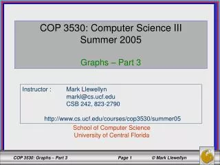
COP 3530: Computer Science III Summer 2005 Graphs – Part 3

COP 3530: Computer Science III Summer 2005 Graphs – Part 3 Instructor : Mark Llewellyn markl@cs.ucf.edu CSB 242, 823-2790 http://www.cs.ucf.edu/courses/cop3530/summer05 School of Computer Science University of Central Florida

One of the first label-correcting algorithms was developed by Lester Ford. Ford’s algorithm is more powerful than Dijkstra’s in that it can handle graphs with negative weights (but it cannot handle graphs with negative weight cycles). To impose a certain ordering on monitoring the edges, an alphabetically ordered sequence of edges is commonly used so that the algorithm can repeatedly go through the entire sequence and adjust the current distance of any vertex if it is needed. The graph shown on slide 4 contains negatively weighted edges but no negative weight cycles. Ford’s Label Correcting Shortest Path Algorithm

As with Dijkstra’s algorithm, Ford’s shortest path algorithm also uses a table via dynamic programming to solve shortest path problems. We’ll run through an example like we did with Dijkstra’s algorithm so that you can get the feel for how this algorithm operates. We’ll examine the table at each iteration of Ford’s algorithm as the while loop updates the current distances (one iteration is one pass through the edge set). Note that a vertex can change its current distance during the same iteration. However, at the end, each vertex of the graph can be reached through the shortest path from the starting vertex. The example assumes that the initial vertex was vertex c. Ford’s Label Correcting Shortest Path Algorithm (cont.)

1 a b 2 5 1 4 4 c d e f 1 1 1 1 1 g 1 i h Graph to Illustrate Ford’s Shortest Path Algorithm Graph for Ford’s Shortest Path Algorithm Example

Ford’s Label Setting Algorithm Ford (weighted simple digraph, vertex first) for all vertices v currDist(v) = ; currDist(first) = 0; while there is an edge (vu) such that [currDist(u) > currDist(v) + weight( edge(vu))] currDist(u) = currDist(v) + weight(edge(vu));

Notice that Ford’s algorithm does not specify the order in which the edges are checked. In the example, we will use the simple, but very brute force technique, of simply checking the adjacency list for every vertex during every iteration. This is not necessary and can be done much more efficiently, but clarity suffers and we are concerned about the technique at this point. Therefore, in the example the edges have been ordered alphabetically based upon the vertex letter. So, the edges are examined in the order of ab, be, cd, cg, ch, da, de, di, ef, gd, hg, if. Ford’s algorithm proceeds in much the same way that Dijkstra’s algorithm operates, however, termination occurs not when all vertices have been removed from a set but rather when no more changes (based upon the edge weights) can be made to any currDist( ) value. The next several slides illustrate the operation of Ford’s algorithm for the negatively weighted digraph on slide 4. Ford’s Label Correcting Shortest Path Algorithm (cont.)

Initially the currDist(v) for every vertex in the graph is set to . Next the currDist(start) is set to 0, where start is the initial node for the path. In this example start = vertex c. Edge ordering is: ab, be, cd, cg, ch, da, de, di, ef, gd, hg, if. The initial table is shown on the next slide. Initial Table for Ford’s Algorithm

iteration  initial 1 vertices  a  b  c 0 d  e  f  g  h  i  Initial Table for Ford’s Shortest Path Algorithm

Since the edge set is ordered alphabetically and we are assuming that the start vertex is c, then the first iteration of the while loop in the algorithm will ignore the first two edges (ab) and (be). The first past will set the currDist( ) value for all single edge paths (at least), the second pass will set all the values for two-edge paths, and so on. In this example graph the longest path is of length four so only four iterations will be required to determine the shortest path from vertex c to all other vertices. The table on slide 11 shows the status after the first iteration completes. Notice that the path from c to d is reset (as are the paths from c to f and c to g) since a path of two edges has less weight than the first path of one edge. This is illustrated in the un-numbered (un-labeled) column. First Iteration of Ford’s Algorithm

With the start vertex set as C, the first iteration sets the following: edge(ab) sets nothing edge(be) sets nothing edge(cd) sets currDist(d) = 1 edge(cg) sets currDist(g) = 1 edge(ch) sets currDist(h) = 1 edge(da) sets currDist(a) = 3 since currDist(d) + weight(edge(da)) = 1+ 2 = 3 edge(de) sets currDist(e) = 5 since currDist(d) + weight(edge(de)) = 1+ 4 = 5 edge(di) sets currDist(i) = 2 since currDist(d) + weight(edge(di)) = 1+ 1 = 2 edge(ef) sets currDist(f) = 9 since currDist(e) + weight(edge(ef)) = 5+ 4 = 9 edge(gd) resets currDist(d) = 0 since currDist(d)+ weight(edge(gd)) = 1+ (-1) = 0 edge(hg) resets currDist(g) = 0 since currDist(g)+ weight(edge(hg)) = 1+ (-1) = 0 edge(if) resets currDist(f) = 3 since currDist(i) + weight(edge(if)) = 2+ 1 = 3 First Iteration of Ford’s Algorithm (cont.)

iteration  initial 1 vertices  A  3 3 B    C 0 D  1 0 E  5 5 F  9 3 G  1 0 H  1 I  2 2 Table After First Iteration currDist(d) is initially set at 1 since edge (cd) is considered first. Subsequently, when considering edge (gd) the currDist(d) can be reduced due to a negative weight edge and currDist(d) becomes 0.

Notice that after the first iteration the distance from vertex c to every other vertex, except b has been determined. This is because of the order in which we ordered the edges. This means that the second pass will possibly set the distance to vertex b but the distance to all other vertices can only be reset if a new path with less weight is encountered. First Iteration of Ford’s Algorithm (cont.)

The second iteration (second pass through edge set) sets the following: edge(ab) sets currDist(b)= 4 since currDist(a) + weight(edge(ab)) = 3+ 1 = 4 edge(be) resets currDist(e)=-1 since currDist(b)+weight(edge(be)) = 4 +(-5) = -1 edge(cd) no change currDist(d) = 0 edge(cg) no change currDist(g)= 0 edge(ch) no change currDist(h) = 1 edge(da) resets currDist(a) = 2 since currDist(d) + weight(edge(da)) = 0+ 2 = 2 edge(de) no change currDist(e)= -1 edge(di) resets currDist(i) = 1 since currDist(d) + weight(edge(di)) = 0 + 1 = 1 edge(ef) no change currDist(f) = 3 edge(gd) resets currDist(d)= -1 since currDist(d)+ weight(edge(gd))= 0+ (-1) = -1 edge(hg) no change currDist(g) = 0 edge(if) resets currDist(f) = 2 since currDist(i) + weight(edge(if)) = 1+ 1 = 2 Second Iteration of Ford’s Algorithm

iteration  initial 1 2 vertices  A  3 3 2 B    4 C 0 D  1 0 1 E  5 5 1 F  9 3 2 G  1 0 H  1 I  2 2 1 Table After 2nd Iteration

The third iteration makes the following updates to the table: edge(ab) resets currDist(b)= 3 since currDist(a) + weight(edge(ab)) = 2+ 1 = 3 edge(be) resets currDist(e)=-2 since currDist(b)+weight(edge(be)) = 3 +(-5) = -2 edge(cd) no change currDist(d) = -1 edge(cg) no change currDist(g)= 0 edge(ch) no change currDist(h) = 1 edge(da) resets currDist(a) = 1 since currDist(d) + weight(edge(da))= (-1)+ 2 = 1 edge(de) no change currDist(e)= -2 edge(di) resets currDist(i) = 0 since currDist(d) + weight(edge(di)) = -1 + 1 = 0 edge(ef) resets currDist(f) = 2 since currDist(e) + weight(edge(ef)) = -2 + 4 = 2 edge(gd) no change currDist(d)= -1 edge(hg) no change currDist(g) = 0 edge(if) resets currDist(f) = 1 since currDist(i) + weight(edge(if)) = 0+ 1 = 1 Third Iteration of Ford’s Algorithm

iteration  initial 1 2 3 vertices  A  3 3 2 1 B    4 3 C 0 D  1 0 1 E  5 5 1 2 F  9 3 2 1 G  1 0 H  1 I  2 2 1 0 Table After 3rd Iteration

The fourth iteration makes the following updates to the table: edge(ab) resets currDist(b)= 2 since currDist(a) + weight(edge(ab)) = 1+ 1 = 2 edge(be) resets currDist(e)=-3 since currDist(b)+weight(edge(be)) = 2 +(-5) = -3 edge(cd) no change currDist(d) = -1 edge(cg) no change currDist(g)= 0 edge(ch) no change currDist(h) = 1 edge(da) no change currDist(a) = 1 edge(de) no change currDist(e)= -3 edge(di) no change currDist(i) = 0 edge(ef) no change currDist(f) = 1 edge(gd) no change currDist(d)= -1 edge(hg) no change currDist(g) = 0 edge(if) no change currDist(f) = 1 Fourth Iteration of Ford’s Algorithm

iteration  initial 1 2 3 4 vertices  A  3 3 2 1 B    4 3 2 C 0 D  1 0 1 E  5 5 1 2 3 F  9 3 2 1 G  1 0 H  1 I  2 2 1 0 Table After 4th Iteration

A fifth and final iteration is needed (its not shown in the table) which upon ending will terminate the algorithm as no changes will be made to the table on the fifth iteration. Since the fourth iteration reset only the currDist( ) for vertices b and e, the only possible changes that could be made to the table during the fifth iteration would be to those same vertices again since these two did not affect the distance to any other vertex during the previous iteration. The fifth and final iteration is shown below: edge(ab) no change currDist(b)= 2 edge(be) no change currDist(e)=-3 edge(cd) no change currDist(d) = -1 edge(cg) no change currDist(g)= 0 edge(ch) no change currDist(h) = 1 edge(da) no change currDist(a) = 1 edge(de) no change currDist(e)= -3 edge(di) no change currDist(i) = 0 edge(ef) no change currDist(f) = 1 edge(gd) no change currDist(d)= -1 edge(hg) no change currDist(g) = 0 edge(if) no change currDist(f) = 1 Fourth Iteration of Ford’s Algorithm

As you can see having stepped through the execution of Ford’s algorithm, the run-time is dependent on the size of the edge set. Ford’s algorithm works best if the graph is sparse and less well if the graph is relatively dense. Comments on Ford’s Shortest Path Algorithm

A vertex represents an airport and stores the three-letter airport code An edge represents a flight route between two airports and stores the mileage of the route 849 PVD 1843 ORD 142 SFO 802 LGA 1743 337 1387 HNL 2555 950 1233 LAX 1120 DFW MCO Graph: Example

NW 35 DL 247 AA 49 DL 335 AA 1387 AA 523 AA 41 1 UA 120 AA 903 UA 877 TW 45 E V BOS LAX DFW JFK MIA ORD SFO Edge List • The edge list structure simply stores the vertices and the edges into two containers (ex: lists, vectors etc..) • each edge object has references to the vertices it connects. Easy to implement. Space = O(n+m) Finding the edges incident on a given vertex is inefficient since it requires examining the entire edge sequence. Time: O(m)

a b c e d a c b d b a e c a e d d a c e e c b d Adjacency List (traditional) • adjacency list of a vertex v: sequence of vertices adjacent to v • represent the graph by the adjacency lists of all the vertices Space =  (n +  deg(v)) = (n + m)

NW 35 DL 247 AA 49 DL 335 AA 1387 AA 523 AA 41 1 UA 120 AA 903 UA 877 TW 45 E V BOS LAX DFW JFK MIA ORD SFO in out in out in out in out in out in out in out NW 35 AA 49 UA 120 AA1387 DL335 NW 35 AA1387 DL 247 AA523 UA 120 UA 877 TW 45 DL 247 AA 41 1 UA 877 AA 49 AA 903 AA 903 AA 41 1 DL 335 AA 523 TW 45 Adjacency List (modern) • The adjacency list structure extends the edge list structure by adding incidence containers to each vertex. space is O(n + m).

a b c d e a b a F T T T F b T F F F T c T F F T T c d T F T F T e F T T T F d e d Adjacency Matrix (traditional) • matrix M with entries for all pairs of vertices • M[i,j] = true means that there is an edge (i,j) in the graph. • M[i,j] = false means that there is no edge (i,j) in the graph. • There is an entry for every possible edge, therefore: Space = (n2)

Adjacency Matrix (modern) • The adjacency matrix structures augments the edge list structure with a matrix where each row and column corresponds to a vertex.

A procedure for exploring a graph by examining all of its vertices and edges. Two different techniques: Depth First traversal (DFT) Breadth First Traversal (BFT) Graph Traversal

Depth-First Search • Depth-first search (DFS) is a general technique for traversing a graph • A DFS traversal of a graph G • Visits all the vertices and edges of G • Determines whether G is connected • Computes the connected components of G • Computes a spanning forest of G

A B D E C A A A B D E B D E B D E C C C Example unexplored vertex A visited vertex A unexplored edge discovery edge back edge

A A A B D E B D E B D E C C C A B D E C Example(cont.)

The algorithm uses a mechanism for setting and getting “labels” of vertices and edges DFS Algorithm AlgorithmDFS(G, v) Input graph Gand a start vertexv of G Output labeling of the edges of G in the connected component of v as discovery edges and back edges setLabel(v, VISITED) for alle  G.incidentEdges(v) ifgetLabel(e) = UNEXPLORED w opposite(v,e) if getLabel(w) = UNEXPLORED setLabel(e, DISCOVERY) DFS(G, w) else setLabel(e, BACK) AlgorithmDFS(G) Input graph G Output labeling of the edges of G as discovery edges and back edges for allu  G.vertices() setLabel(u, UNEXPLORED) for alle  G.edges() setLabel(e, UNEXPLORED) for allv  G.vertices() ifgetLabel(v) = UNEXPLORED DFS(G, v)

Property 1 DFS(G, v) visits all the vertices and edges in the connected component of v Property 2 The discovery edges labeled by DFS(G, v) form a spanning tree of the connected component of v A B D E C Properties of DFS

Setting/getting a vertex/edge label takes O(1) time Each vertex is labeled twice once as UNEXPLORED once as VISITED Each edge is labeled twice once as UNEXPLORED once as DISCOVERY or BACK DFS runs in O(n+m) time provided the graph is represented by the adjacency list structure Analysis of DFS

DFS on a graph with n vertices and m edges takes O(n + m ) time DFS can be further extended to solve other graph problems Find and report a path between two given vertices Find a cycle in the graph Depth-First Search

COP 3530: Computer Science III Summer 2005 Graphs – Part 3